Four-point bending tests on T-beams
Introduction
This section analyzes an experimental investigation involving four-point bending tests performed on T-beams by Leonhardt and Walther (1963). This experimental campaign comprised 18 tests conducted on reinforced concrete beams with constant geometry and varying reinforcement layouts for the stirrups. Specimens TA9, TA10, TA11 and TA12 (with vertical stirrups and varying 6. EXPERIMENTAL VALIDATION | 105 reinforcement amounts) were chosen for comparison with results gained from the CSFM, since they cover a wide range of failure modes from shear to flexural.
Definition of failure modes
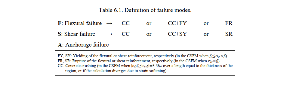
In order to compare the observed failure modes in the experiments with those predicted by the CSFM, the failure modes are classified as follows: flexural (F), shear (S) and anchorage (A). It should be noted that none of the experiments covered in this chapter exhibited an anchorage failure. Table 6.1 defines different failure subtypes depending on whether flexural and shear fail-ures are triggered by failure of the concrete or of the reinforcement. While yielding of the reinforcement does not represent a material failure, this is included as a failure subtype in combination with concrete crushing due to the importance of distinguishing concrete crushing failures without reinforcement yielding (very brittle) from those happening after the yielding of the reinforcement (which can exhibit a certain deformation capacity).
Experimental setup
All of the investigated beams had the same geometry and reinforcement arrangements, as shown in Fig. 6.1. The beam span (spacing between the supports) was 3000 mm. The flanges had a width of 960 mm and a depth of 80 mm. The webs had a width of 160 mm, and the total depth of the beams was 440 mm. Each of the two applied loads (P/2) was applied at a distance of 1250 mm from the supports, which resulted in a spacing between loads of 500 mm. The flexural reinforcement consisted of six reinforcing bars of 24 mm in diameter. Four longitudinal reinforcing bars with a diameter of 10 mm were placed in the flange. Open stirrups with hooked ends at the top (see Fig. 6.1a) were used as shear reinforcement; these were always placed at a spacing of st = 113 mm. The only parameter that varied between specimens TA9, TA10, TA11 and TA12 was the diameter (Øt) of the stirrups, which led to different geometric reinforcement ratios (ρt,geo) (see Table 6.2).
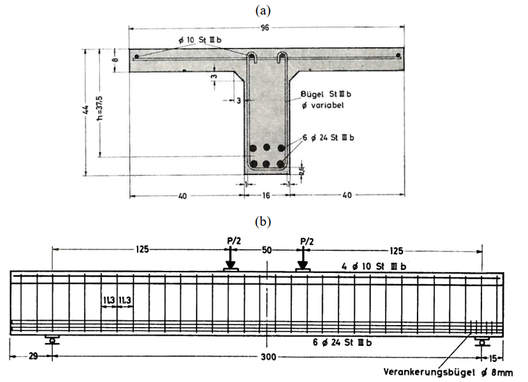
Table 6.2. Relevant parameters of the analyzed specimens.

1) ρcr calculated with Eq. f ρ considering fct = 1.9 MPa
\[ρ_{\text{cr}} = \frac{f_{\text{ct}}}{f_{\text{y}} - (n-1)f_{\text{ct}}}\]
where:
- \(f_y\) - reinforcement yield strength
- \(f_{ct}\) - concrete tensile strength
- \(n = \frac{E_s}{E_c}\) - modular ratio
Material properties
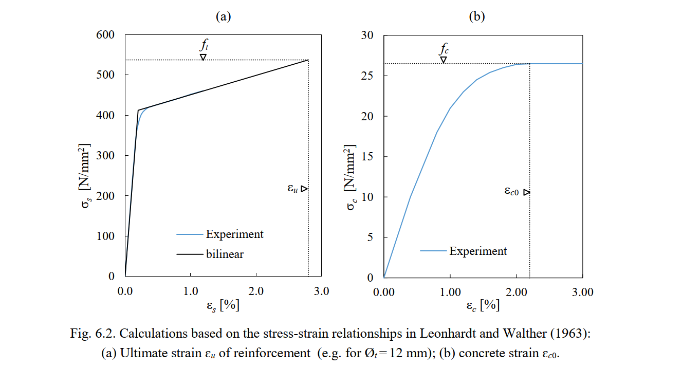
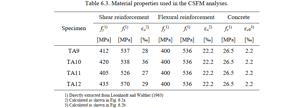
The material properties of the concrete and reinforcement used in the CSFM analysis are summarized in Table 6.3. The modulus of elasticity (Es), the yield stress (fy) and the ultimate stress (ft) of the reinforcement as well as the compressive strength (fc) of the concrete are directly extracted from the experimental report (Leonhardt and Walther 1963). This report only provides the experimental stress-strain relationships of the reinforcing bars up to a strain of 12 ‰. The ultimate strain of the bare reinforcement (εu) is estimated based on the known experimental values (fy, ft and incomplete stress-strain relationships) and assuming a bilinear response. Fig. 6.2a illustrates this estimate for the case of Øt = 12 mm. The values obtained for the failure strain εu for all used diameters are given in Table 6.3. The compressive strain of concrete at peak stress (ɛc0, see Fig. 3.1c) is directly extracted from the experimental concrete stress-strain relationship (see Fig. 6.2b)
Modeling with the CSFM
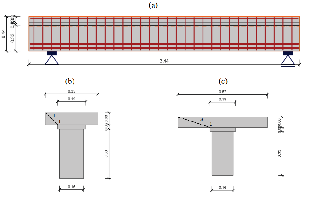
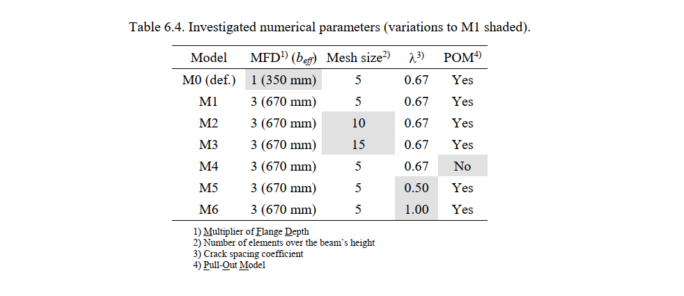
The geometry, reinforcement, supports and loading conditions were modeled in the CSFM according to the experimental setup (see Fig. 6.3a). Several numerical calculations were carried out using different values for the following parameters:
- The multiplier of the flange depth (MFD), which is the inverse of the slope considered for the expansion of the compression field into the flange (see Figure 6.3) to account for the shear lag effect (see Section 3.6.3). The MFD coefficient was set to 1.0 (default value in IDEA StatiCa Detail) and 3.0 (slightly above the recommendation of the fib Model Code 2010 for this specific configuration). These settings define the effective flange width (beff), which yield to beff = 350 mm and beff = 670 mm, respectively (Figure 6.3b-c).
- The consideration or not of potentially non-stabilized cracking in stirrups. When considered (by default), the Pull-Out Model (POM) defines tension stiffening in stirrups with geometric reinforcement ratios below (ρcr) (Eq. (3.5)), while the Tension Chord Model (TCM) is used for other bars and stirrups above (ρcr). When deactivated, the models account for tension stiffening by means of the TCM in all cases.
- The mesh size, which was 5 (the default value in IDEA StatiCa Detail for this particular example), 10 or 15 finite elements over the beam’s depth. The default mesh is very coarse in this geometry (i.e., designers should avoid using fewer than four finite elements in a cross section); therefore, only finer meshes than the default one are analyzed in this study.
- The crack spacing coefficient (λ) was varied to consider minimum (λ = 0.5), average (λ = 0.67, default value) and maximum crack spacing (λ = 1.0). This parameter affects the tension stiffening behavior of reinforcing bars with stabilized crack patterns (see Section 3.3.4)
Table 6.4 shows the parameters used in each numerical calculation (model M0 to M6). M0 corresponds to the model with the default settings in the CSFM. As will be discussed in Section 6.2.4, the default value of the multiplier of the flange depth was too conservative in this case and led to an excessively soft response. Therefore, the default value (MFD = 1; beff = 350 mm) was only used in M0. In the other models, the MFD was set to 3 (beff = 670 mm).
Comparison with experimental results
This section provides comparisons between the experimental results and the ultimate loads and failure modes provided by the CSFM. In order to also verify the use of the CSFM for serviceability behavior, the load-deformation response and crack patterns predicted by the numerical analyses are compared with those from the tests. Furthermore, the measured and calculated crack widths are compared for specimens TA9 and TA12, which exhibited flexural and shear failures, respectively.
Failure modes and ultimate loads
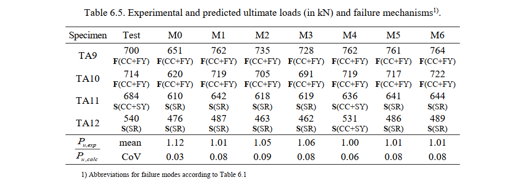
Table 6.5 summarizes the ultimate loads measured in the tests (Pu,exp), the ultimate loads predicted by the CSFM (Pu,calc), and the respective failure modes. P denotes the total applied force. This table also provides the mean and the coefficient of variation (CoV) of the ratios between the measured and the calculated ultimate loads for each numerical model. Ratios above one denote conservative predictions of the ultimate load. As seen in Table 6.5, the basic failure modes in all CSFM analyses agree with the experimental results, but differences in the failure subtypes are observed in some cases for Specimen TA11, and in one case for TA12. The predictions of the ultimate loads given by the default model (M0) are very satisfactory, yielding slightly conservative results (12% on average) with a very small scatter among the analyzed beams.
The differences among the CSFM analyses can be easily analyzed in Fig. 6.4, where the ratios of experimental and calculated ultimate loads (Pu,exp/Pu,calc) are shown. Increasing the effective flange width from the default value (MFD = 1; beff = 350 mm) in model M0 to the value specified by the fib (International Federation for Structural Concrete 2013) (MFD = 3; beff = 670 mm) in model M1 led to an increase in the ultimate loads (Fig. 6.4a). The influence of the flange width was very small in those tests where failure in shear occurred (TA11 and TA12), but significant (up to 14%) in the case of bending failures (TA9 and TA10). The consideration of an increased effective flange width (model M1) led on average to better results than with the default model, but at the cost of a larger scatter. Hence, M1 is used in Fig. 6.4 as the reference model for the following comparative analyses.
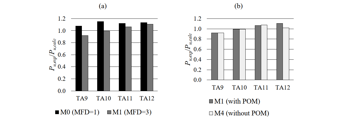
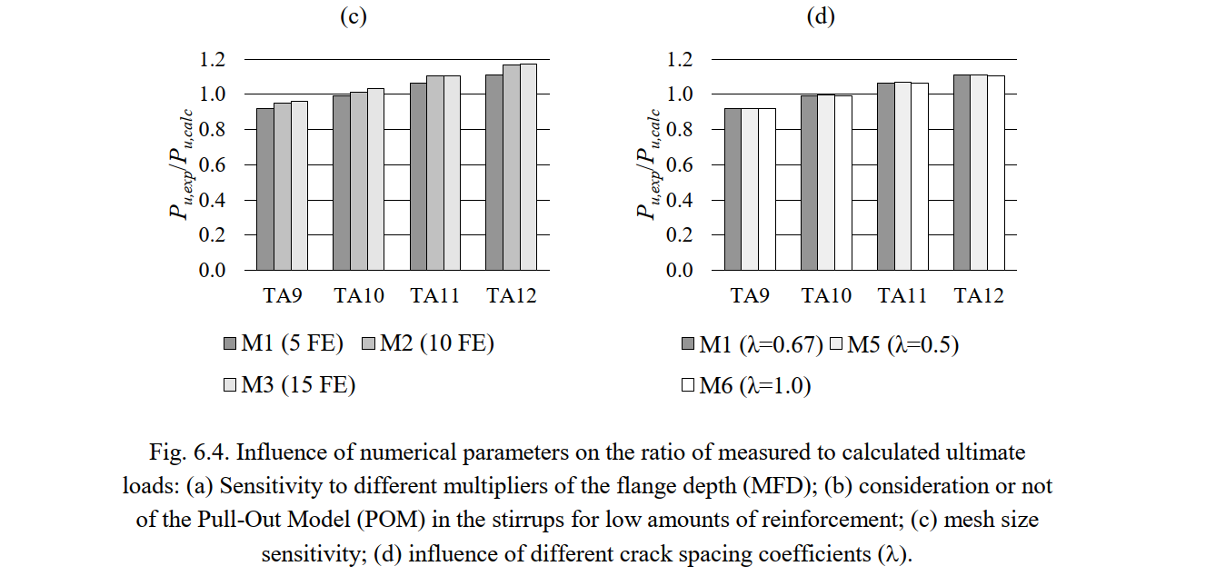
The results of the consideration or not of potentially non-stabilized cracking in stirrups are shown in Fig. 6.4b. This parameter only affected the results for Specimens TA11 and TA12 (TA9 and TA10 have a large amount of stirrups – ρt,geo > ρcr, see Table 6.2 – and therefore tension stiffening was accounted for by using the Tension Chord Model (TCM) regardless of this setting). In numerical model M1, the tension stiffening of TA11 and TA12 was modeled with the Pull Out Model (POM), but the TCM was used in M4. Using the POM or the TCM had a small impact on the strength predictions in this particular case (a maximum of 10% for TA12), since the amount of stirrups is quite high in all cases. The consideration of the POM is more relevant when modeling structural elements with a lower amount of stirrups, as will be discussed in Section 6.4. The influence of the mesh size and the crack spacing parameters on the ultimate load was very small in this case (the differences are below 5%, see Fig. 6.4c-d).
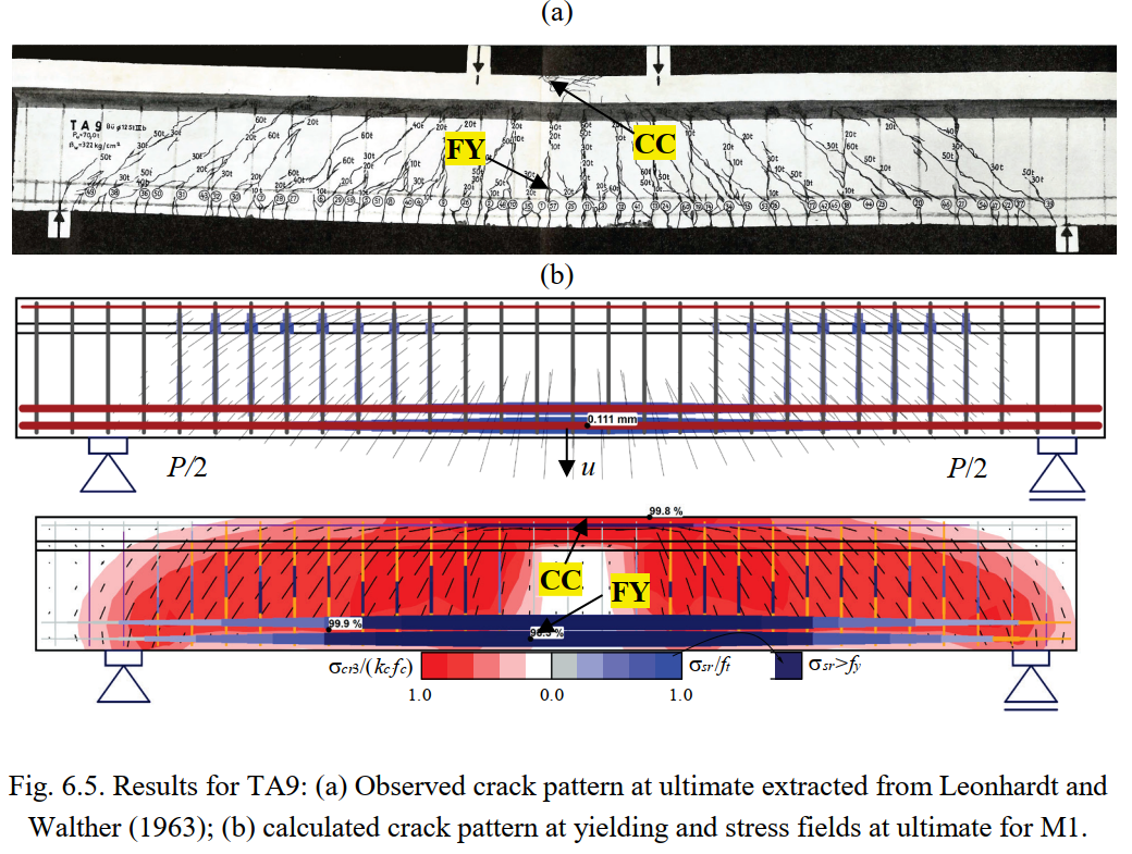
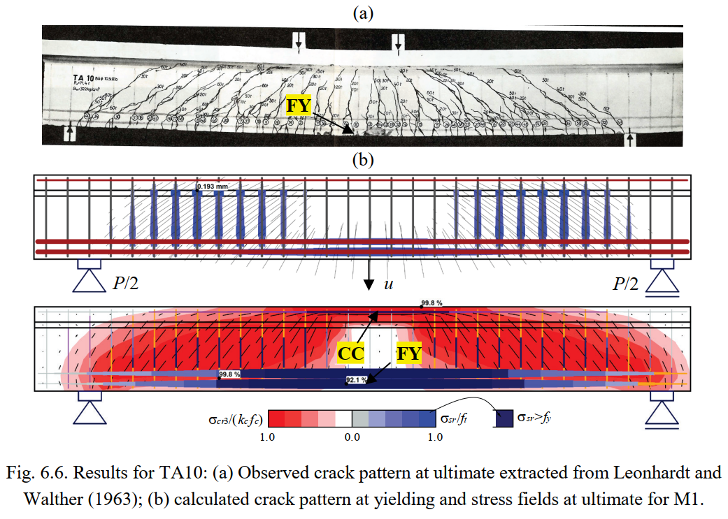
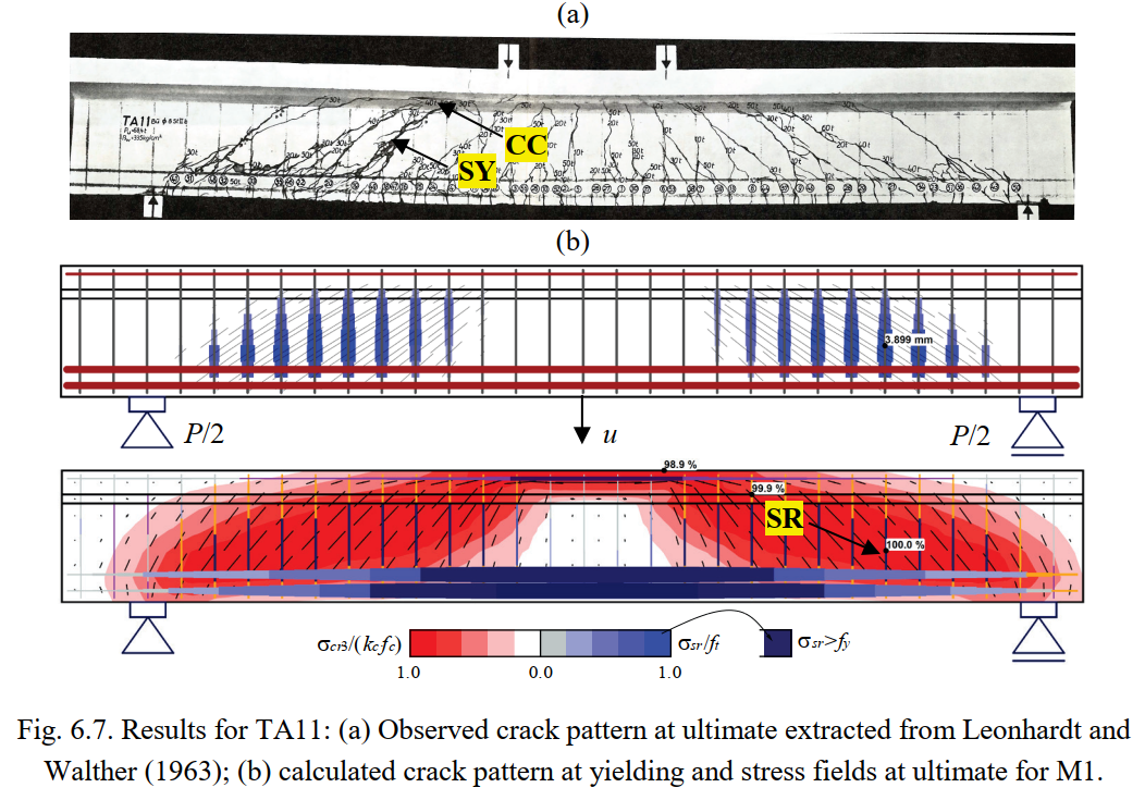
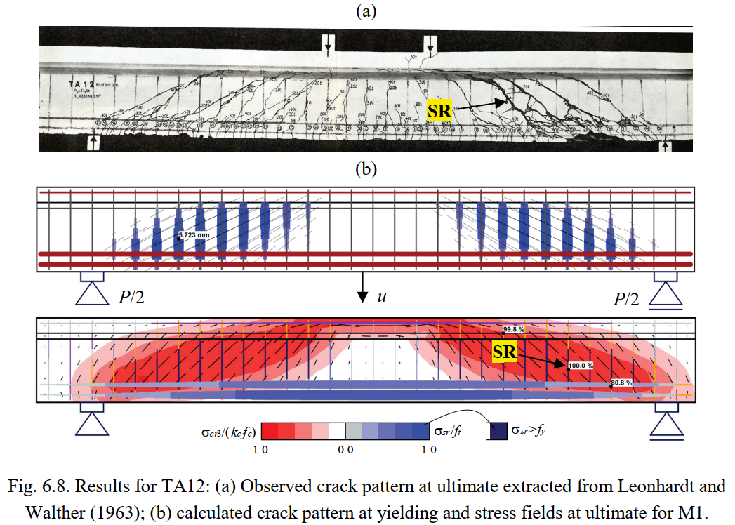
Figures 6.5 to 6.8 show the resulting stress fields and the identification of failure modes. In Figures 6.5a to 6.8a, the observed failure modes are marked on top of the photos of the tested specimens (for TA10 the reported concrete crushing in bending is not marked since it is not evident in the photo). The failure modes predicted by the numerical model M1 are highlighted in Figures 6.5c to 6.8c, which show the stress fields at ultimate limit state, including the principal compressive stresses (σcr3) and the steel stresses (σsr) at the cracks. M1 corresponds to the default parameters, except for the effective flange width, which is based on the fib Model Code 2010 (International Federation for Structural Concrete 2013). The predicted failure modes agree fairly well with the experimental observations, including their location. The model of Beam TA11 is slightly conservative since it predicts a failure of the stirrups, while only their yielding is reported in the experiments. The calculation of cracked regions and the magnitudes of the crack widths (represented by the length of the lines) at the onset of yielding are plotted in Figures 6.5b to 6.8b. The numerical parameters from M1 are also used in this case. The predicted cracked regions and crack orientations agree well with the experimental observations at failure in Figures 6.5a, 6.6a, 6.7 and 6.8a.
Load-deformation response
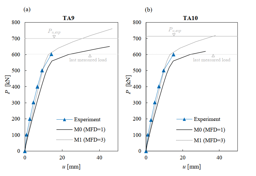
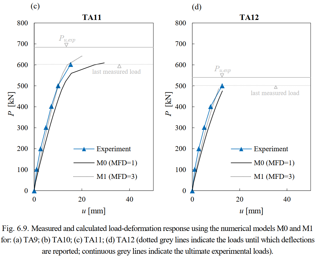
Fig. 6.9 shows the measured load-deformation response as well as the calculated responses using the default numerical parameters (Model M0 with MFD = 1 and beff = 350 mm) and the increased flange width according to the fib Model Code 2010 (Model M1 with MFD = 3 and beff= 670 mm). The load-deformation responses predicted by the other analyzed models (M2 to M6) are very similar to those from model M1 and not shown here. The value of the load P corresponds to the total applied force and u corresponds to the deflection at midspan (see e.g., Fig. 6.5b). Leonhardt and Walther (1963) did not report complete load-deformation responses. Hence, the graphs contain two grey horizontal lines: (i) a dashed line indicating the maximum load for which deflections were reported and (ii) a continuous line indicating the ultimate experimental load.
A good agreement was found between the calculated load-deformation response and the experimental results in all tests within the range of the available measurement data. While the calculation using default parameters (M0) is slightly too soft, the use of an increased flange depth (M1) provides an excellent agreement. The comparison of the predictions of the load-deformation response shows that it is possible to realistically capture very different deformation capacities, as obtained in the tests depending on the amount of shear reinforcement.
Crack widths at service loads
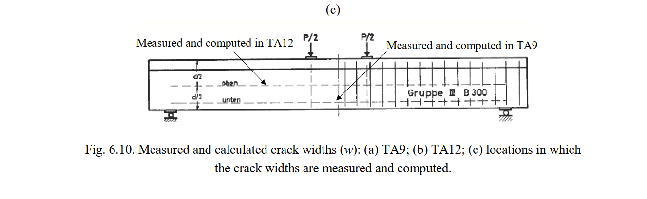
Fig. 6.10a-b compares the crack widths (w) predicted by the CSFM with the maximum values reported by Leonhardt and Walther (1963). Two tests with different failure modes are studied in this comparison: Test TA9 (flexural failure) and TA12 (shear failure). The crack widths were measured for the flexural reinforcement in TA9 and in the middle of the web in TA12 (see Fig. 6.10c). As stated in Section 3.5.4, the models used to calculate crack widths are only valid if the reinforcement remains elastic. Hence, the crack width results in Fig. 6.10 are given only up to the yielding load. It should be noted that the first crack width measurement for specimen TA12 was performed after yielding. Hence, Fig. 6.10b does not show any measuring point, just the linear interpolation up to the first measurement. The predictions were carried out using the numerical models M1, M5 and M6, which only differ in the crack spacing coefficients used for the crack width calculation: λ = 0.67 (mean), λ = 0.5 (minimum) and λ = 1.0 (maximum).
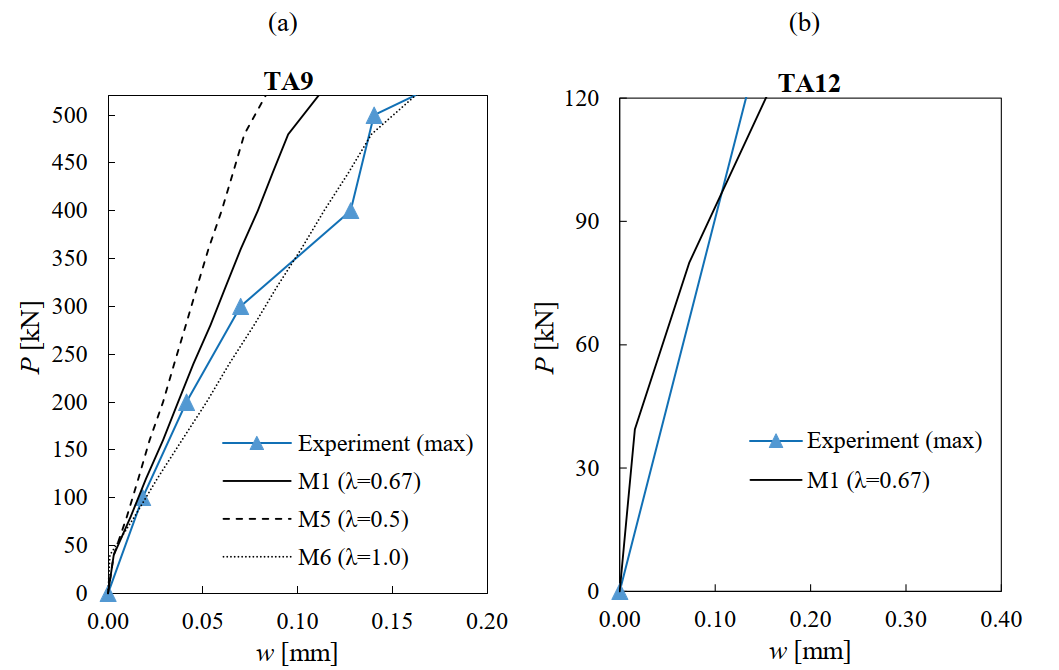
The numerical results for TA9 predict the measured bending crack widths very well (see Fig. 6.10a). The CSFM results for the maximum crack widths (M6 with crack spacing coefficient λ = 1) agree excellently in this case with the observed maximum crack widths. As expected, a decreasing crack spacing coefficient (λ) leads to smaller crack widths. However, the crack widths calculated in regions with non-stabilized cracking (as in the web of TA12, see Fig. 6.10b) are independent of the crack spacing coefficient, since the calculation does not rely in this case on crack spacing (see Fig. 3.10e). The calculated crack widths in regions with non-stabilized cracking should be interpreted as good estimates of the maximum expected crack widths. Fig. 6.10b shows the predicted crack widths in the web of TA12, which match the measured maximum crack widths fairly well. As already mentioned, only the range in which all reinforcement remains elastic is shown, since only in this range the CSFM provides appropriate crack width results.
Conclusions
A good correspondence is found between the results from the CSFM and the experimental observations. The following conclusions can be stated:
- The use of the default parameters in IDEA StatiCa Detail leads to slightly conservative estimates of ultimate loads, load-deformation response and failure modes.
- The analysis of the sensitivity of the model to parameters different from the default ones shows that the most relevant parameter in this case is the considered value of the effective flange width. Designers can change the default width by inputting the geometry via a wall or general shape templates. The larger effective flange width provided by the fib Model Code 2010 leads to very accurate estimates of the experimental ultimate loads, deflections and crack widths.
- The consideration of tension stiffening by means of the Pull Out Model in the beam with the lowest amount of stirrups predicts an ultimate load that errs on the safe side by around 10%. When using the Tension Chord Model, the experimental failure mode cannot be properly captured. This mismatch can impact the accuracy of the ultimate load predictions particularly for low amounts of stirrups.
- The crack spacing coefficient and the mesh size do not significantly affect ultimate loads and failure modes. The crack spacing coefficient only has a significant influence on the crack width results of those reinforcing bars in which the Tension Chord Model is used for tension stiffening.