Cantilever wall-type bridge piers
Introduction
This article is dedicated to the simulation via the CSFM of the load-deformation response of three out of seven cantilever wall-type bridge pier experiments performed by Bimschas (2010) and Hannewald et al. (2013). These experiments were conducted under a vertical constant load, combined with a cyclic (but quasi-static) horizontal force. The design and detailing of the specimens was similar to that of existing bridge piers with seismic deficiencies. Specimens VK1, VK3 and VK6 were selected for analysis with the CSFM. These specimens had different amounts of flexural reinforcement and shear slenderness (achieved by varying the height of the walls). It should be noted that the CSFM just aims at describing the envelope of the cyclic response (so-called “backbone”) using a monotonic model.
Definition of failure modes
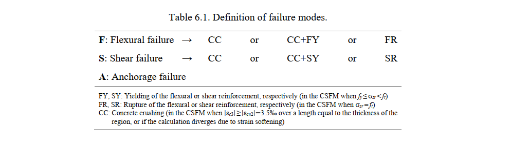
In order to compare the observed failure modes in the experiments with those predicted by the CSFM, the failure modes are classified as follows: flexural (F), shear (S) and anchorage (A). It should be noted that none of the experiments covered in this chapter exhibited an anchorage failure. Table 6.1 defines different failure subtypes depending on whether flexural and shear fail-ures are triggered by failure of the concrete or of the reinforcement. While yielding of the reinforcement does not represent a material failure, this is included as a failure subtype in combination with concrete crushing due to the importance of distinguishing concrete crushing failures without reinforcement yielding (very brittle) from those happening after the yielding of the reinforcement (which can exhibit a certain deformation capacity).
Experimental setup
All piers were 1500 mm deep and 350 mm wide. The total height (H) of specimens VK1 and VK3 was 3700 mm, and that of VK6 was 4850 mm, see Fig. 6.11. The specimens stood on a stiff foundation block, which will not be modeled in the CSFM.
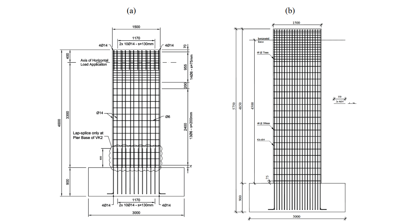

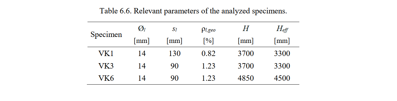
In all tests, a constant vertical load of 1370 kN was applied to the top of the piers. After the vertical force was applied, the specimens were subjected to a horizontal cyclic load (V) applied quasi-statically at an effective height above the foundation block of Heff = 3300 mm in the case of VK1 and VK3 and Heff = 4500 mm for VK6. The application of the horizontal load was displacement-controlled. The flexural reinforcement (vertical direction) consisted of continuous reinforcing bars with a diameter of Øl = 14 mm distributed along the cross-section with a spacing sl of 130 mm for VK1 and 90 mm for VK3 and VK6. The resulting geometric reinforcement ratios ρl,geo are summarized in Table 6.6. The flexural reinforcement was anchored at the foundation (anchor-age length of 200 mm plus end hooks). All specimens had the same shear reinforcement (horizontal direction) consisting of hoops of diameter Øt = 6 mm at a spacing of st = 200 mm. This resulted in a very low shear reinforcement ratio of ρl,geo = 0.08 % (which is below the critical reinforcement ratio according to
\[ρ_{\text{cr}} = \frac{f_{\text{ct}}}{f_{\text{y}} - (n-1)f_{\text{ct}}}\]
where:
- \(f_y\) - reinforcement yield strength
- \(f_{ct}\) - concrete tensile strength
- \(n = \frac{E_s}{E_c}\) - modular ratio).
The stirrup spacing was reduced to 75 mm at the region where load was applied (top of the pier). Relevant parameters are stated in Table 6.6.
Material properties
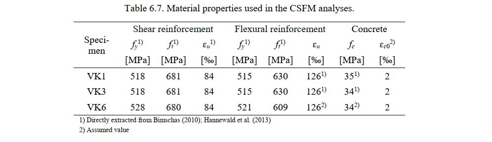
Table 6.7 summarizes the material properties used in the CSFM analysis, which are based on the material tests carried out by Bimschas (2010) and Hannewald et al. (2013). The properties not provided in these reports (the ultimate strain of the flexural reinforcement ɛu and the concrete strength fc for VK6, as well as the concrete strain at peak load ɛc0 for all tests) were assumed to be as indicated in Table 6.7 (expected mean values for materials used).
Modeling with the CSFM
The geometry, reinforcement, supports and loading conditions were modeled in the CSFM according to the experimental setup (see Fig. 6.12).
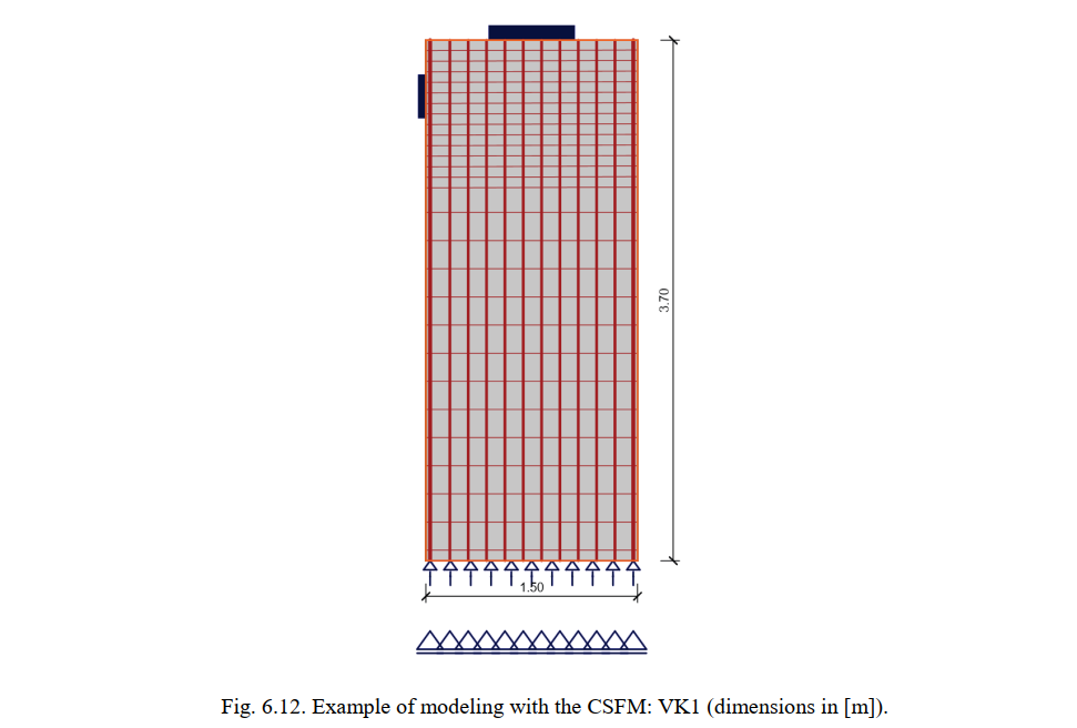
The foundation was not included in the model. To simulate the fixed-end support properly, the flexural bars were anchored outside of the concrete region and the anchorage length was not verified in the calculation. Several numerical calculations were carried out using different values for the following parameters:
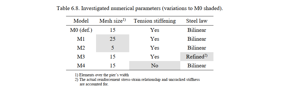
- The mesh size, which was 5, 15 (the default value in IDEA StatiCa Detail for this particular example) and 25 finite elements along the wall’s width.
- The consideration or not of the tension stiffening effect. By default tension stiffening (TS) is considered in the CSFM.
- The stress-strain relationship for the reinforcement. By default, a bilinear stress-strain relationship is used in the CSFM. A refined analysis was also performed considering the actual stress-strain relationship of the reinforcement (cold-worked for the flexural and hot-rolled for the shear reinforcement) and accounting for the initial uncracked stiffness. This refined behavior was simulated via a user-defined reinforcement stress-strain relationship.
The parameters used in each numerical calculation (model M0 to M4) are summarized in Table 6.8. Model M0 corresponds to the default settings in the CSFM.
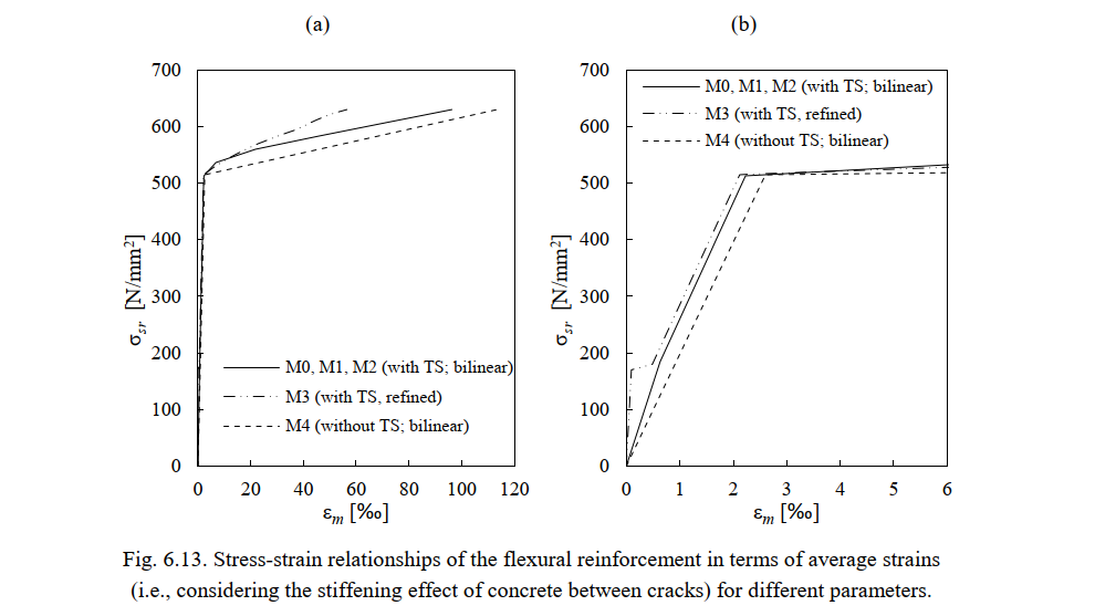
An example of the influence of the used parameters on the response of the reinforcement (including the tension stiffening effect) is illustrated in Fig. 6.13 for the flexural reinforcement. The consideration of the uncracked stiffness is reflected in the elastic part of these diagrams.
Comparison with experimental results
The ultimate shear force (i.e., the horizontal applied load), the failure modes and the load-deformation response determined by the CSFM are compared with the corresponding experimental results below.
Failure modes and ultimate loads
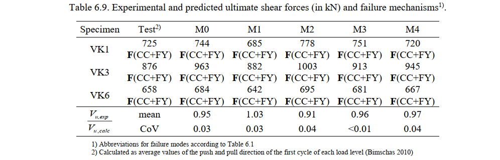
The ultimate shear forces predicted by the CSFM (Vu,calc) and measured in the experiments (Vu,exp), and the respective failure modes, are summarized in Table 6.9. This table also provides the mean and the coefficient of variation (CoV) of the ratios between measured and calculated ultimate loads for each numerical model. Ratios above one denote conservative predictions of the ultimate load. As seen from Table 6.9, the failure mechanisms of all tests were predicted well by the CSFM, independently of the used parameters. The default model M0 leads to slightly unsafe strength predictions (on average 5%): A minor issue, which can be solved by using a finer mesh.
The sensitivity of the strength predictions of the CSFM to the different analyzed numerical parameters is shown in Fig. 6.14 by means of the ratio of experimental to calculated ultimate shear forces (Vu,exp/Vu,calc). The strength predictions show a moderate mesh size sensitivity in these tests (see Fig. 6.14a). A decrease in mesh size leads to a decrease in the computed ultimate loads. However, the predicted failure modes remain insensitive to the considered mesh size (see Table 6.9). The difference in the ultimate loads when using 5 (Model M2) or 25 (Model M1) elements over the width of the wall is up to 12%. Moreover, the ultimate load is nearly independent of the consideration or not of tension stiffening (see Fig. 6.14b), or the use of a refined stress-strain relationship for the reinforcement (see Fig. 6.14c). In the analyzed experiments, these effects only have a relevant influence on the stiffness of the members, as will be shown below.
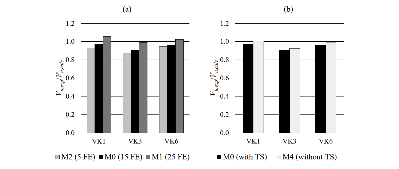
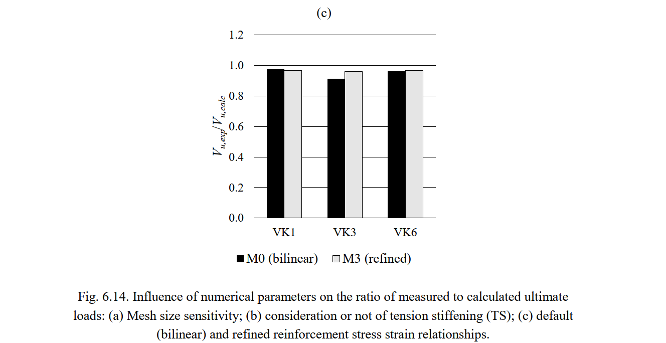
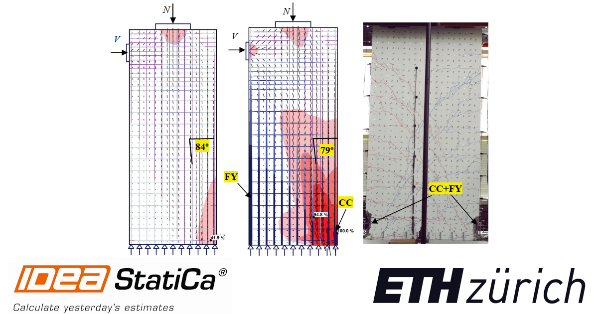
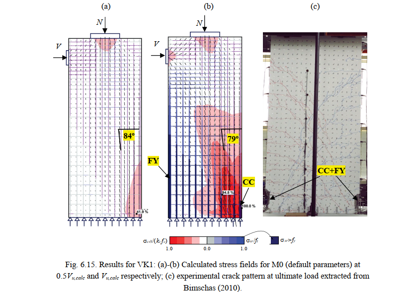
Fig. 6.15a-b shows the continuous stress field results in Specimen VK1 provided by the CSFM for two load steps (0.5Vu,calc and Vu,calc). These results were calculated using default numerical parameters (M0). It can be seen that due to plastic redistributions, the compression field was significantly steeper (more inclined with respect to the vertical wall axis) at ultimate. The predicted failure mode (concrete crushing with yielding of the flexural reinforcement) is highlighted in Fig. 6.15b. The location agrees with the experimental observations (highlighted in Fig. 6.15c, where it can be seen that the cyclic loading produced concrete crushing in both sides).
Load-deformation response
Fig. 6.16 shows a comparison of the calculated load-deformation response provided by the CSFM with the envelope (backbone) of the cyclic response of the experiments. The experimental response was calculated as average values of the push and pull direction of the first cycle of each load level (Bimschas 2010). The numerical predictions were calculated using the following numerical parameters: Default parameters (M0), refined stress-strain relationship of the reinforcement (M3), and neglecting tension stiffening (M4). The reference experimental displacement u was obtained by subtracting the part due to anchorage slip from the total measured displacement at the height at which load was applied. This allows a direct comparison with the numerical results since the foundation is not modeled in the CSFM analysis. The contribution of anchorage slip was evaluated following the assumptions given in Bimschas (2010).
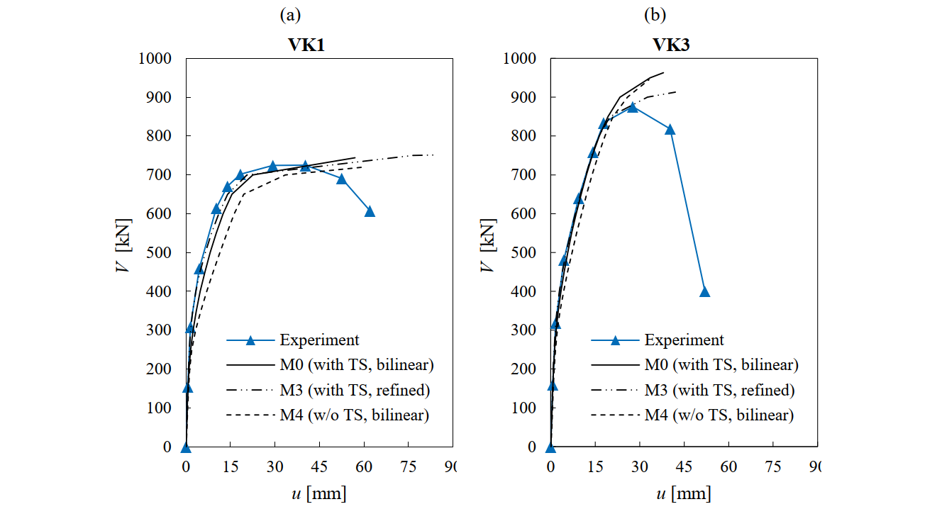
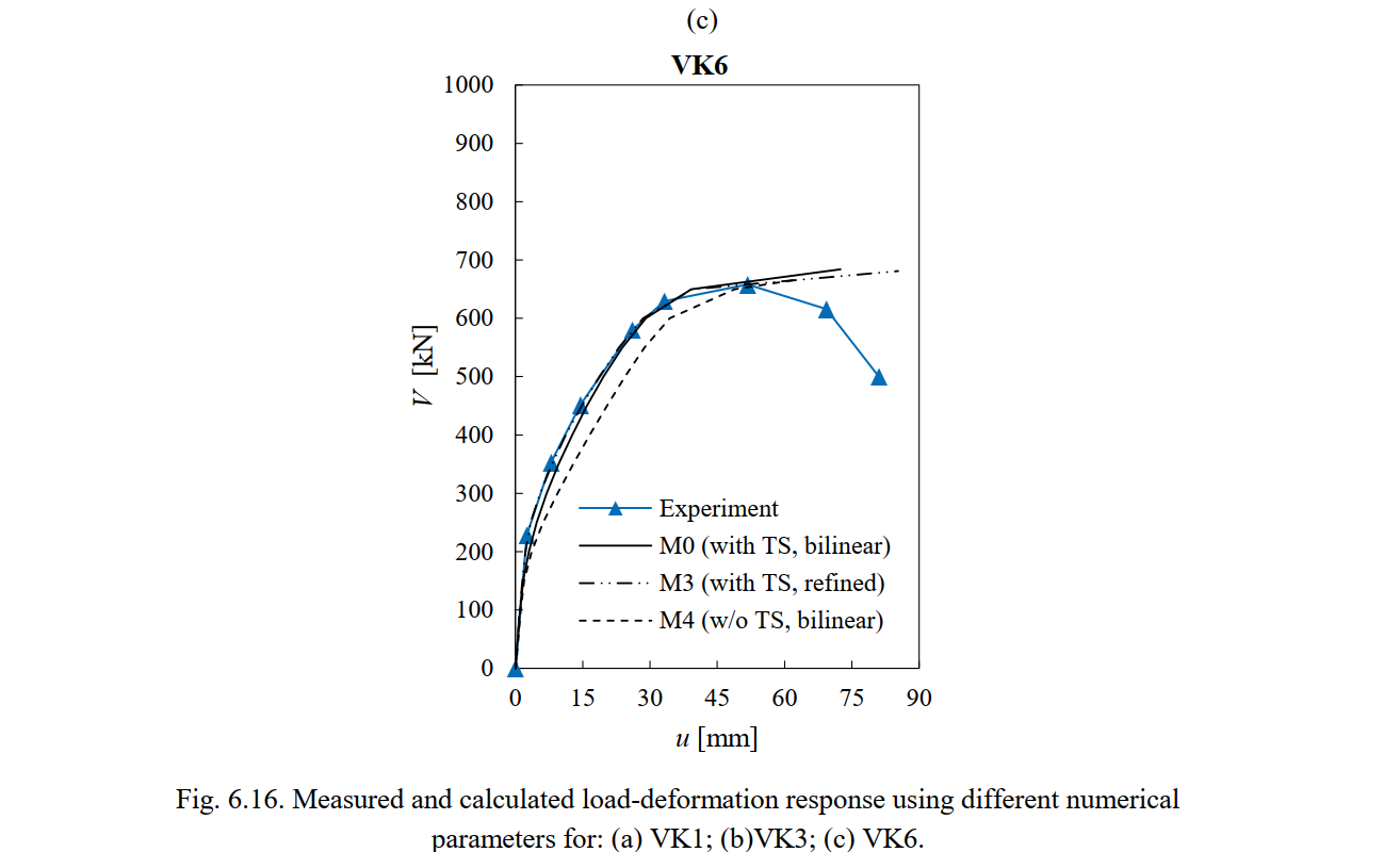
The results in Fig. 6.16 show that it is essential to account for tension stiffening if one needs to have a good estimate of a member’s stiffness. Both numerical calculations considering tension stiffening (M0 and M3) fit the experimental results very well. However, the behavior was too soft when this effect was neglected (M4), particularly for VK1 and VK6. The consideration of the actual stress-strain relationship of the reinforcement (hot-rolled and cold-worked) and the uncracked stiffness of the reinforcement (model M3) improved the already accurate load-deformation prediction obtained with the default parameters, leading to excellent agreement with the experimental data up to the peak load. The load-deformation response shows very small sensitivity to the analyzed range of finite element mesh sizes (the results for M1 and M2 are very similar to the results with a default mesh size and are not plotted in Fig. 6.16). Hence, it can be concluded that the mesh size only affects the load bearing capacity but not the deformations in this particular case.
It should be noted that the CSFM does not account for the concrete softening after reaching peak load (instead, a code compliant plastic plateau is implemented). Clearly, the intention of the CSFM is not to capture the softening branch of the experiments. Still, it provides a good estimate of the deflection in the post-peak phase, during which a significant amount of load-bearing capacity is lost (i.e., to give a good estimate of the deformation capacity of the structural members). The results with default parameters (model M0) in Fig. 6.16 show that the numerical analyses detected the failure for a displacement at which the specimens had lost around 15% of their maximum strength. This is a good estimate of the deformation capacity and highlights the capabilities of the CSFM besides the implementation of simple and code-compliant constitutive relationships.
Conclusions
As in the tests analyzed in Section 6.2, a good agreement can be found between the predictions given by the CSFM and the experiments, showing that the model exhibits only a small sensitivity to changes in the parameters. The following conclusions can be stated:
- Using the default parameters implemented in IDEA StatiCa Detail results in the CSFM slightly overestimating the ultimate load (by 5% on average), which might be attributed to the cyclic loading in the experiments causing progressive damage. Hence, the CSFM provides appropriate predictions of ultimate loads but also failure modes.
- The CSFM predictions exhibit moderate changes when the size of the finite element mesh varies significantly. In this case, refining the default mesh leads to better estimation of the ultimate loads. Therefore, it is highly recommended that the sensitivity of the model to changes in the mesh size should always be investigated.
- The tension stiffening effect has no influence on ultimate load, but is essential for the proper estimation of deflections and deformation capacity.
- Using a refined stress-strain relationship for the reinforcement and considering the uncracked stiffness of the walls leads to excellent deflection predictions. For design purposes, it is recommended that the default simplified bilinear relationship be used, as it also provides good estimates of deflections, slightly on the safe side.