IDEA StatiCa RCS – Structural design of 1D concrete members

Design of reinforced concrete sections according to EN 1992-1-1 and EN 1992-2.

Bending
Shear
Torsion
Interaction
Stress limitation check
Crack control
N-M-κ diagram
Literature

Bending

Methods for sectional capacity check

Two well-known methods can be used to check the ultimate limit state for 1D concrete members. The first one will give us the cross-sectional ultimate strength in the form of an interaction area or an interaction diagram (in the case of bending moment in one direction). Cross-sectional capacity can be determined as the ratio of acting internal forces to limit state forces. The second one is finding equilibrium in a cross-section, where we are looking for the actual behaviour of the loaded section, the use of materials in terms of stresses, and insight into the vulnerabilities of the section.

General design assumptions and calculation assumptions for Ultimate Limit State 

1. Strain ε in the reinforcement and concrete shall be assumed directly proportional to the distance from the neutral axis (plane sections remain plane).
2. Interaction of the reinforcement and concrete is ensured by concrete and reinforcement interaction without slip (strain ε supports the strain in concrete adjacent fibers are the same).
3. The tensile strength of concrete is neglected (all tensile stresses are transmitted by the reinforcement).
4. Concrete compression stresses in the compression zone are calculated in relation to the strain calculated from stress-strain diagrams.
5. Reinforcement stresses are calculated in relation to the strain from stress-strain diagrams.
6. Compressive concrete strain with an ultimate strain limit ε_cu2 (Parabola-rectangle diagram for concrete under compression) and ε_cu3 (Bi-linear stress-strain relation), [2].
7. The compressive strain of reinforcement is without limitation in the case of the horizontal plastic top branch, in the case of the inclined plastic top branch the strain is limited ε_ud,[2].
8. A limit state is considered when the state of at least one of the materials exceeds the ultimate limit strain (if εu is not limited, the compressed concrete is governing).

\[ \textsf{\textit{\footnotesize{\qquad Strain stress.}}}\]

\[ \textsf{\textit{\footnotesize{\qquad Stress-strain design diagram for reinforcing steel with inclined top branch.}}}\]

Interaction diagram

The first option is to check the cross-section by an interaction surface (or interaction diagram). An explanation is provided on a sample of the interaction surfaces for the reinforced square section from the example in the figure below. On the interaction surface are located points defining the ultimate limit state of the examined cross-section. The interaction surface is drawn from the points (N, My, Mz), which are determined by stress integration in the cross-section, which has achieved ultimate limit strain in one of the materials. For a 3D  interaction, the surface can be derived from a 2D interaction diagram, which is a closed curve, which corresponds to the stress of a constantly rotated neutral axis.

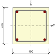
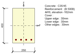
\[ \textsf{\textit{\footnotesize{\qquad Symmetrical reinforced cross-section.}}}\]

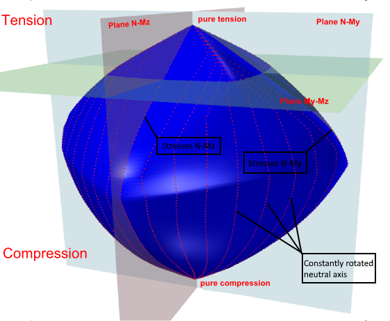
\[ \textsf{\textit{\footnotesize{\qquad Interaction surface shows failure conditions for all load cases of normal force and bending moments.}}}\]

For the case of a symmetrical cross-section about the y-axis, the interaction diagram is symmetrical around the plane N-M_y. Identically, for the case of a symmetrical cross-section about the z-axis, the interaction diagram is symmetrical around plane N-M_y. The one-sided reinforced section introduces a flattened shape of the interaction diagram

\[ \textsf{\textit{\footnotesize{\qquad Single symmetrical reinforced cross-section.}}}\]

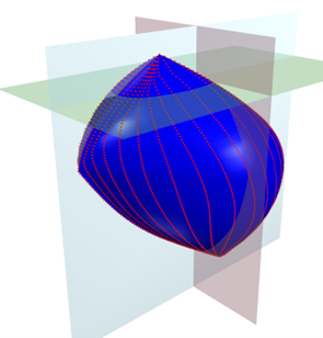
\[ \textsf{\textit{\footnotesize{\qquad Interaction surface for cross-section with single symmetric reinforcement.}}}\]

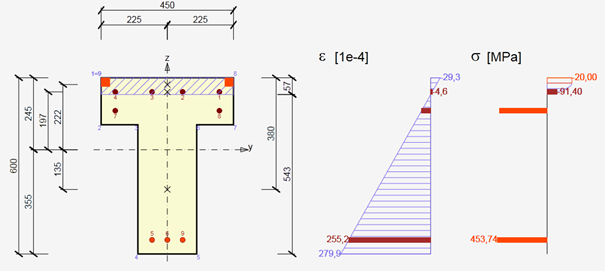
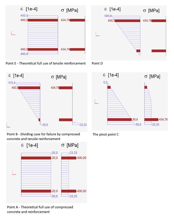
The points defining the ultimate limit state are received from stress integration.  The figure below displays strain at the ultimate limit state.

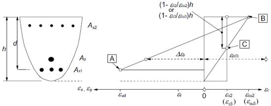
\[ \textsf{\textit{\footnotesize{\qquad Strain distributions at the ultimate limit state (taken from [2]).}}}\]

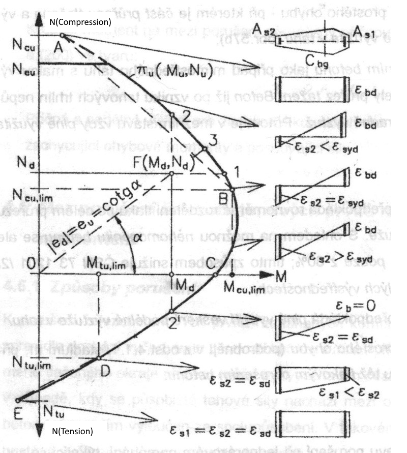
The interaction diagram shows cross-section failure under normal force and bending moments. [1]

Respecting the 2D diagram problem (closed curve laying on interaction surface) we can find out the strain plane is passing through the neutral axis and critical point [y, z, ε], which is considered as critical point R.  Point [y, z] defines a point in cross-section with the value of strain ε at the ultimate limit state. The neutral axis inclination is constant for all points of the 2D diagram.

In case the compressive stress in concrete is critical for design, point R is matching the farthest compressed concrete fiber or to limiting point C. However, this can be applied only if that section is made from one type of concrete - not such as a mixed cross-section.   

In the case the tensile stress in reinforcement is critical for design (strain ε_ud is exceeded at the ultimate limit state for one or more bars), there must be fulfilled condition that for the given strain plane the value ε_ud is not exceeded at any other bar.

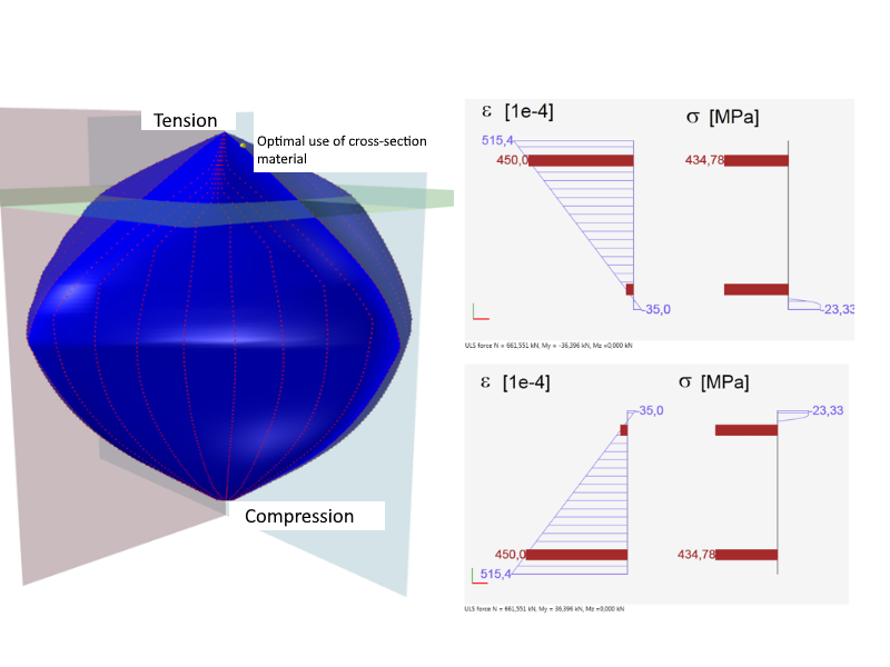
\[ \textsf{\textit{\footnotesize{\qquad Optimal use of cross-section material.}}}\]

\[ \textsf{\textit{\footnotesize{\qquad Characteristic strain plane positions calculated for purpose of interaction diagram.}}}\]

The picture above shows that the diagram can be divided into two parts: the part where the failure is caused by tensile force and the part which fails by a compressive force. The limit points correspond to the case above, where the extreme inclination of the strain plane also can be seen. When drawing an interaction diagram the plane strain inclination of a cross-section is changing in this interval, while we search for the point R (see above). Based on that defined plane we perform the integration to get the stress at the ultimate limit state.

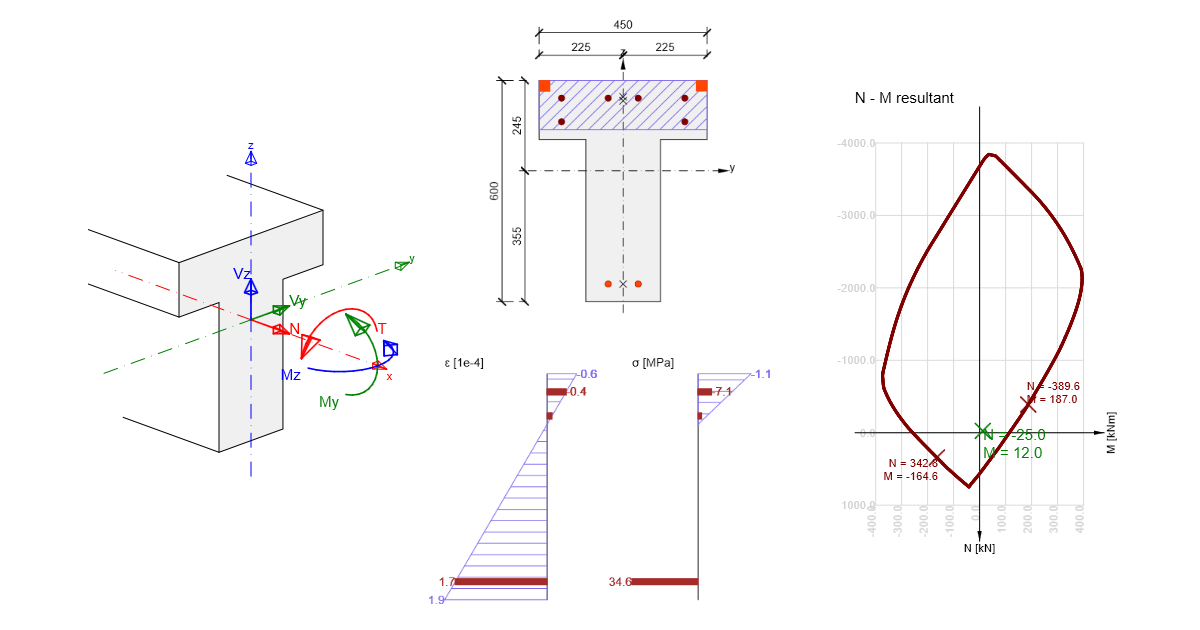
Cross-section subjected to axial force and bending moment check

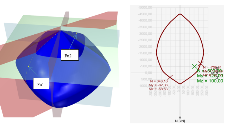
The check of a cross-section subjected to axial force and bending moment relies in proving that the checked stresses (combination N_d, M_zd, M_zd) are located inside or on the surface interaction area. Different methods can do this. The following example demonstrates the check of a rectangular cross-section subjected to forces N_d = -500 kN, M_yd = 120 kNm, M_zd = 100 kNm.

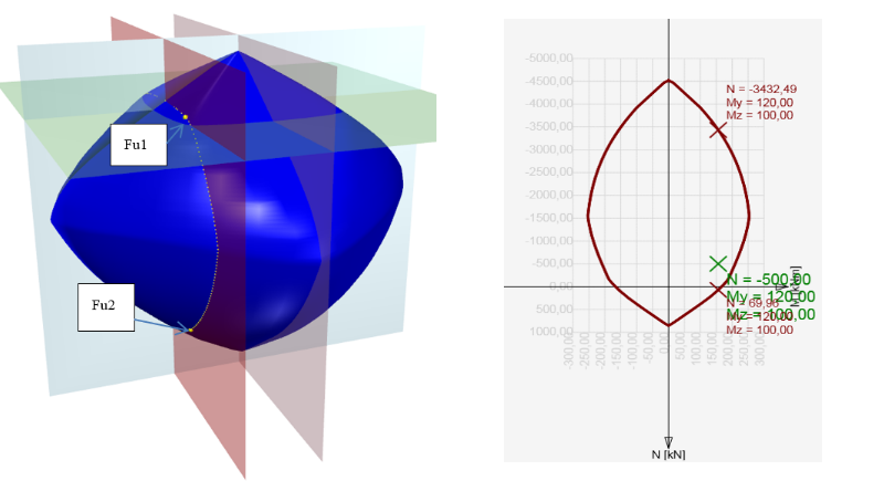
Method NuMuMu

To define the resistance of a cross-section we assume proportional changes in all of the internal force components (the eccentricity of the normal force remains constant) until the interactive surface has been developed. The change of involved internal forces can be interpreted as moving along a line connecting the start coordinate system (0,0,0) and the point defined by the internal forces (N_Ed, M_Ed,y, M_Ed,z). The two intersections of this line with the interaction surface, which can be found, represents two sets of forces at the ultimate limit state. At each intersection, the program determines three forces at the limit state: the design axial force resistance N_Rd and the corresponding design moments of resistance M_Rdy, M_Rdz.

Method  NuMM

To define the resistance of cross-section we assume constant normal force (which is equal to the acting design normal force) and proportional changes in bending moments until the interactive surface has been developed. The change of involved internal forces can be interpreted as moving in a horizontal plane along the line connecting the point (N_Ed,0,0) and the  point defined by the acting internal forces (N_Ed, M_Ed,y, M_Ed,z). The two intersections of this line with the interaction surface, which can be found, represents two sets of forces at the ultimate limit state. At each intersection the program determines three forces at the limit state: the design resisting moments M_Rdy, M_Rdz and (corresponding) acting design normal force N_Ed.

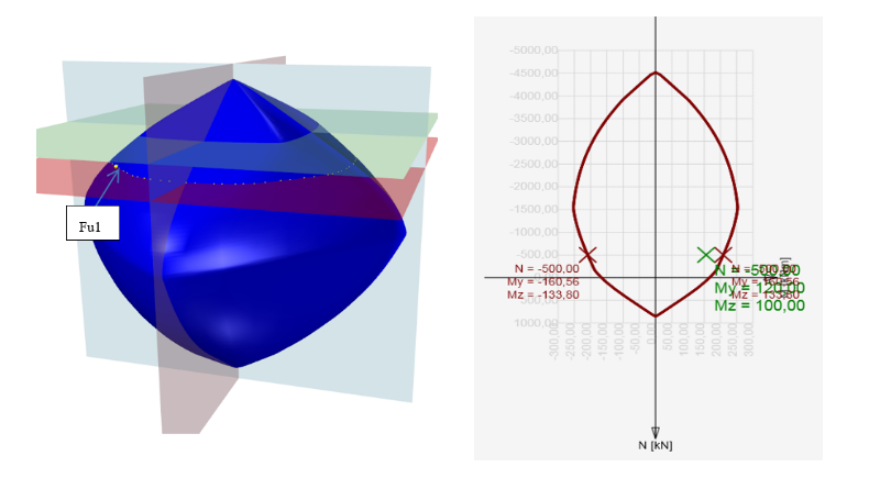
Method  NMuMu

To define the resistance of the cross-section we assume a constant normal force (which is equal to the acting design normal force) and proportional changes in bending moments until the interactive surface has been developed. The change of the involved internal forces can be interpreted as moving in a horizontal plane along the line connecting the point (N_Ed,0,0) and the point defined by the acting internal forces (N_Ed, M_Ed,y, M_Ed,z). The two intersections of this line with the interaction surface, which can be found, represent two sets of forces at the ultimate limit state. At each intersection, the program determines three forces at the limit state: the design resisting moments M_Rdy, M_Rdz, and (corresponding) acting design normal force N_Ed.

Finding the section response

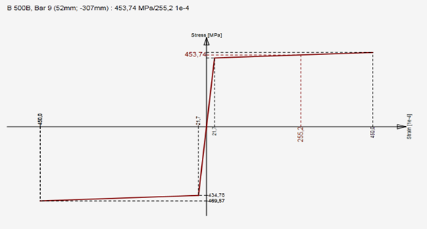
Another possibility to check the cross-section is by finding the cross-section response (i.e. Strain and stress distribution from acting internal forces). This method is also known as the method of limit deformation. The level of acting stresses in each fiber (in the case of plane bending in each layer) in each reinforced bar is calculated depending on the strain of the Stress-strain diagram of the material.
Finding the cross-section response is calculated using the numerical method specified in [6]. The principle consists of the gradual load increment of the section by the unbalanced components of not-transferred forces. Those are obtained by integrating the stress over the section using Stress-strain diagrams. If the stress value can be found for the strain in the Stress-strain diagram, see Figure below (a), the calculated stress is correct assuming linear elastic material. In cases (b) and(c), the stress for a linear calculation reaches unrealistic values, and part (b) or entire value (c) cannot be transmitted by the material. Integrating not-transferred stresses we get not-transferred internal forces, and their resultants should be added to the internal forces of variable loads. 

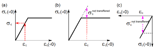
Not-transferred stresses in Stress-strain diagrams. [4]

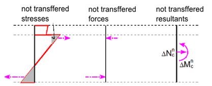
Not-transferred inner forces. [4]

This calculation method requires the use of numerical methods for integrating the stress over the cross-section area and for nonlinear analysis of equilibrium equations in the section. Iteration is terminated at the time when the convergence criteria are met.

\[\frac{{{F_e} - {F_i}}}{{{F_e}}} \le max\left\{ {e,d} \right\}\]

where 

F_e is section load,

F_i is section response (internal forces calculated on the base of the strain plane).

If a is the approximate (approximated) value and b is the exact (true) value, then absolute deviation is given by the following equation.

\[e = \left| {b - a} \right|\]

Relative deviation is given by the following formula:

\[d = \left| {\frac{{b - a}}{b}} \right|\]

In most programs, you can set these convergence criteria (default values are 1% as relative error, 100 N, 100 Nm as the absolute error of normal force and moments). 

So if we have the input of N = 0 kN, My = 100 kNm, Mz = 0 kNm and integrated forces after iteration N = - 0.07 kN, My = 100.5 kNm, Mz = 0.02 kNm, the evaluation will be as follows. With respecting the N and Mz being equal to 0, a comparison with absolute deviation can be done:

The value of normal force 100N> | 70 | N
The value of the bending moment Mz 100Nm> | 20 | Nm
The value of the bending moment My

\[d = \left| {\frac{{b - a}}{b}} \right| = \frac{{100 - 100,5}}{{100}} = 0,005\; < 0,01\]

Cross-section check by the response

In the case of finding a balance in the cross-section, plane strain is known. From the plane strain we can calculate strain anywhere in the section, then the stress or inner forces in reinforcement bars, cross-section or its parts using Stress-strain diagrams of the materials. The calculated stress and strain values we compare with the limit strain value from the stress-strain diagrams of the used materials.
The advantage of this method is that we get a complete image of the stress and strain values in the section of the internal forces acting on the cross-section.

Shear

With respect to fragile failure the shear check is one of the important checks of a reinforced concrete section.

Calculation procedure

Calculation of shear resistance is composed of several basic parts. At first we should analyze whether cracks due to bending occur or not in the checked location. If any, use the calculation according to EN 1992-1-1 [2], Article 6.2.2 (1). Otherwise, we determine whether it is plane concrete or poorly reinforced concrete, then proceed in accordance with EN 1992-1-1 Article 12.6.3. 

For reinforced uncracked concrete (without shear reinforcement) we check according to EN 1992-1-1 Article 6.2.2 (2). For Elements, where is required shear reinforcement we check according to Article 6.2.3 [2].

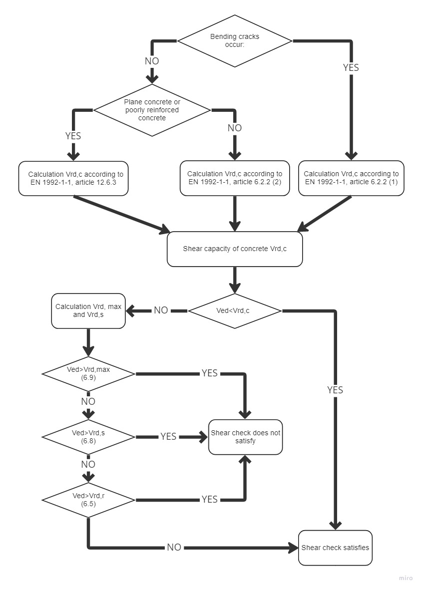
\[ \textsf{\textit{\footnotesize{\qquad Process diagram for shear check.}}}\]

Shear resistance of members without shear reinforcement

Shear resistance of members in cracked bending zones (art. 6.2.2 (1) [2])

Shear resistance of reinforced concrete members without shear reinforcement subject to bending moment is given by:

 \[{{V}_{Rd,cm}}=~{{C}_{Rd.c}}k~{{\left( 100~{{\varrho }_{l}}{{f}_{ck}} \right)}^{{}^{1}/{}_{3}}}~{{b}_{w}}d\]

Which was defined on the base of tests executed on a representative number of simple beams in case of failure by shear force. Since the above resistance may be zero for elements without longitudinal reinforcement (r_l), for poorly reinforced members was derived equations. Since the above resistance may be zero for members without longitudinal reinforcement (r_l), for the poorly reinforced members was determined by equation

\[{{V}_{Rd,c}}\ge ~{{\upsilon }_{min}}{{b}_{w}}d\]

For shear resistance with influence of normal force was determined by equation

\[{{V}_{Rd,cn}}=~{{k}_{1}}{{\sigma }_{cp}}~{{b}_{w}}d\]

Shear resistance in its complete expression which is corresponding with EN 1992-1-1 art. 6.2.2 (1)

\[{{V}_{Rd,c}}=~\left[ {{C}_{Rd.c}}k~{{\left( 100~{{\varrho }_{l}}{{f}_{ck}} \right)}^{{}^{1}/{}_{3}}}+{{k}_{1}}{{\sigma }_{cp}} \right]~{{b}_{w}}d\]

With minimum of

\[{{V}_{Rd,c}}=~\left( {{\upsilon }_{min}}+{{k}_{1}}{{\sigma }_{cp}} \right){{b}_{w}}d\]

where  

C_Rd,c    = 0,18 / γ_c,

k          cross-section height factor 

\[k=1+\sqrt{\frac{200}{d}}<2,0\]

ρ₁      reinforcement ratio for longitudinal reinforcement

\[{{\varrho }_{l}}=\frac{{{A}_{sl}}}{{{b}_{w}}d}\le 0,02\]

f_ck        characteristic compressive cylinder strength of concrete at 28 days

k₁         = 0,15

σ_cp       = N_Ed / A_c < 0,2 f_cd  v MPa

b_w        smallest width of the cross-section in the tensile area

d          effective depth of a cross-section

υ_min      minimal equivalent shear strength υ_min = 0.035 k^3/2 fck^1/2

Shear resistance of members in uncracked bending zones (art. 6.2.2 (2) [2])

Shear resistance of members in uncracked bending zones can be determined from the Mohr circle. Into equation

\[{{\sigma }_{1,2}}=\frac{{{\sigma }_{x}}+{{\sigma }_{y}}}{2}\pm \sqrt{{{\left( \frac{{{\sigma }_{x}}-{{\sigma }_{y}}}{2} \right)}^{2}}+\tau _{z}^{2}}\]

We substitute σ_x = σ_cp a τ_z = V_Rd,c S / (I b_w) and figure out V_Rd,c and get equation corresponding with formula given in EN 1992-1-1 art. 6.2.2 (2)

where  

I           is the second moment of area,

b_w        is the width of the cross-section at the centroidal axis

S          is the first moment of area above and about the centroidal axis,

f_ctd        design axial tensile strength of concrete in MPa,

 s_cp       is the concrete compressive stress at the centroidal axis due to loading and/or prestressing,

a_l         transmission length factor, usually 1,0.

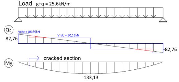
In relation with the above it should be noted that in areas without bending cracks the resistance V_Rd ,c  can be significantly higher than in cracked areas according to Article 6.2.2 (1) [2]. The figure below clearly shows that although the shear force is checked at its extreme (which does not produce cracks), need not necessarily ensure that it will be transferred along the whole beam length. It is due to a change in the method of calculating the shear resistance of the concrete. On the safe side, of course, the shear resistance can be considered according to Article 6.2.2 (1) [2] also in places where cracks will not occur.

\[ \textsf{\textit{\footnotesize{\qquad Shear resistance comparison before and after the cracks occurred.}}}\]

To the expression of V_Rd, c  according to Article 6.2.2 (2)[2] it must also be noted that in the general case should be based on check at the fiber of the extreme principal concrete tensile stress in the zone of normal compressive stress, but not at the center of gravity of the section. At this point it is necessary to calculate the cross-sectional characteristics (S and b_W). To determine the maximum principal stress s₁ in program IDEA RCS we draw a line through the centre of gravity in the direction of the resultant shear forces. This line we divide to 20 sectors. On this line we will present more characteristic points (points of the cross-section polygon, centre of gravity, the neutral axis). Within these points, we calculate S, b_w, σ_x, τ_yz a σ_1.  At the point of maximum principal tensile stress we will calculate the shear resistance.

Shear force before applying the reduction factor b required by Article 6.2.2 (6) must satisfy the extra condition

\[ {{V}_{Ed}}\le 0,5~{{b}_{w}}d~\upsilon ~{{f}_{cd}}\]

where 

 \[ {{ υ}}\le 0,6\left[ 1-\frac{{{f}_{ck}}}{250} \right]\]  kde f_ck je v MPa

Shear resistance of members without reinforcement or lightly reinforced (art. 12.6.3 [2])

Shear resistance for plain or lightly reinforced concrete can be determined from the expression

\[ {{\tau }_{cp}}\le k~{{V}_{Ed~}}/{{A}_{cc}}\]

Where

τ_cp we substitute by

\[ {{f}_{cvd}}=\sqrt{f_{ctd,pl}^{2}+{{\sigma }_{cp}}{{f}_{ctd,pl}}}~pro~{{\sigma }_{cp}}\le {{\sigma }_{c,lim}}~\]

or

\[ {{f}_{cvd}}=\sqrt{f_{ctd,pl}^{2}+{{\sigma }_{cp}}{{f}_{ctd,pl}}-{{\left( \frac{{{\sigma }_{cp}}-{{\sigma }_{c,lim}}}{2} \right)}^{2}}}~pro~{{\sigma }_{cp}}>{{\sigma }_{c,lim}}~\]

Partial values used in the above formula are given by:

\[ {{\sigma }_{c,lim}}={{f}_{cd,pl}}-2\sqrt{{{f}_{ctd,pl}}\left( {{f}_{ctd,pl}}+{{f}_{cd,pl}} \right)}\]

where  

f_cd,pl     Design compressive strength  for plain or lightly reinforced concrete,

f_ctd,pl    Design axial tensile strength of plain or lightly reinforced concrete,

f_cvd       Design shear resistance under concrete compression.

The resistance of members with shear reinforcement (art. 6.2.3 [2])

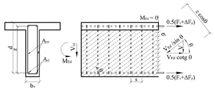
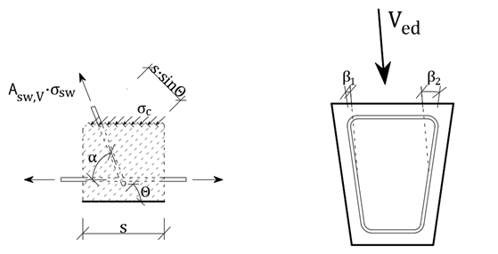
Calculation of reinforced concrete members resistance with shear reinforcement is based on the truss analogy method with variable-angle diagonals. The basis of this method is the balance of forces in the triangle determined by the strut force (diagonal), the shear reinforcement force (stirrup) and longitudinal reinforcement force.

\[ \textsf{\textit{\footnotesize{\qquad Principe of Truss analogy for member under shear load.}}}\]

Cross-section under shear load is broken by cracks at an angle θ, from this reason the concrete diagonal with same angle as shear forces is resisting to the shear force. Compressive force of the diagonal can be expressed as V_ed/sinθ. This force must be transferred by concrete surface, perpendicular to the compression diagonal b_wzcosθ. The concrete tension stress in the compression diagonal is then equal:

\[ {{\sigma }_{c}}=\frac{{{V}_{Ed}}}{{{b}_{w}}z~\sin \text{ }\!\!\theta\!\!\text{ }\cos \theta }=\frac{{{V}_{Ed}}}{{{b}_{w}}z}\left( \tan \theta +\cot \theta  \right)\]

Substituting \[{{\sigma }_{c}}={{\alpha }_{cw}}{{\nu }_{1}}{{f}_{cd}}\]  and \[{{V}_{Ed}}={{V}_{Rd,max}}\] and expressing \[{{V}_{Rd,max}}\] we get equation for  shear resistance of diagonal:

\[ {{V}_{Rd,max}}=~{{\alpha }_{cw}}~{{b}_{w}}~z~{{\nu }_{1~}}{{f}_{cd}}/\left( \cot \theta +\tan \theta  \right)\]

To balance the vertical force component in the compression diagonal, shear reinforcement will be used. The size of the vertical force is based on the diagonal compressive stress in the concrete area which is corresponding to one single stirrup - \[{{\sigma }_{c}}{{b}_{w}}s{{\sin }^{2}}\theta\]. Limit stirrup force is given as \[{{A}_{sw}}{{f}_{ywd}}/s\]. 

Inserting σ_c, comparing with the limit force in the reinforcement, after modifications we get:

\[ \frac{{{A}_{sw}}{{f}_{ywd}}}{s}=\frac{{{V}_{Ed}}}{z}\tan \theta\]

Then expressing V_ed as V_RDs we get resistance of cross-section with vertical shear reinforcement:

\[ {{V}_{Rd,s}}=~\frac{{{A}_{sw}}}{s}z~{{f}_{ywd}}\cot \theta\]

The longitudinal shear force is transferred by longitudinal reinforcement and it can be determined as V_edcotgθ . Derivation of formulas above can be found in [4].

Using the program IDEA RCS it is possible to check only members with vertical shear reinforcement. In general following equations can be used:

\[{{V}_{Rd,s}}=~\frac{{{A}_{sw}}}{s}z~{{f}_{ywd}}\left( \cot \theta +\cot \alpha  \right)\sin \alpha\]

\[{{V}_{Rd,max}}=~{{\alpha }_{cw}}~{{b}_{w}}~z~{{\nu }_{1~}}{{f}_{cd}}\left( \cot \theta +\cot \alpha   \right)/\left( 1+{{\cot }^{2}}\theta  \right)\]

Where  

A_sw      is the cross-sectional area of the shear reinforcement,

s           is the spacing of the stirrups,

f_ywd      is the design yield strength of the shear reinforcement,

b_w        is the minimum width between tension and compression chords. To calculate the resistance V_Rd,max , the value of the section width must be reduced to the so-called nominal width of the cross-section in case the cross-section is weakened by cable ducts

           b_w,nom=b_w-0,5ΣΦ for grouted metal ducts

           b_w,nom=b_w-1,2ΣΦ for non-grouted metal ducts           

υ          = 0,6 pro f_ck ≤ 60MPa or  pro f_ck > 60MPa,

α_cw       is a coefficient taking account of the state of the stress in the compression chord.

Load	σcp = 0	0 < σcp≤0,25 fcd	0,25 fcd < σcp≤0,5 fcd	0,5 fcd < σcp≤1,0 fcd
Coefficient acw	1,0	1+σcp/fcd	1,25	2,5(1 - σcp/fcd)

Tab. 1‑1 Determining coefficient α_cw

Angle θ is the angle between the concrete compression strut and the beam axis perpendicular to the shear force. The limiting values of cotθ for use in a Country may be found in its National Annex. The recommended limits are given by the expression:

\[1~\le ~\cot \theta \le 2,5\]

Choosing the size of the angle θ can affect the value of the resistances. Dependence of resistances is visible in Figure 1.15. The figure shows that with increasing of angle θ the resistance V_Rd,max  is increasing, and resistance V_Rd,s is decreasing. Resistance V_Rd,c is constant, since it is based on the truss analogy method.

\[ \textsf{\textit{\footnotesize{\qquad Dependency between shear resistance and angle q.}}}\]

Cross-section characteristics calculation for shear

To calculate the shear it is important to calculate the cross-sectional variables affecting the shear resistance. These variables include mainly shear-resisting section width b_w, the effective depth d and lever arm z. The code [2] gives these values that directly correlate with the actual bending stress. But the problem is to determine these values when the direction of the resultant bending moments (or more accurately the direction of the resultant of section resistance) is significantly different from the direction of the resultant shear forces. In this case, the EC2 code doesn’t provide any recommendations.

Cross-section width resisting to shear b_w

The IDEA RCS program calculates the cross-section width resistant to shear in the direction perpendicular to the resultant of shear forces. Depending on the article in the Eurocode this width is calculated as:
-  The smallest width of the section between the resultant of compressive concrete and tensile reinforcement in the direction perpendicular to the resultant of shear forces for article 6.2.2 (a) and 6.2.3 (1)
- The section width in a direction perpendicular to the resultant of shear forces in the checked point according to article 6.2.2 (2)

Effective depth of a cross-section

Effective depth is usually defined as the distance of most compressed concrete fiber to the centre of gravity of the reinforcement. Because it is directly related to the bending, the distance is given as perpendicular projection to the gravity line of the plane strain. 

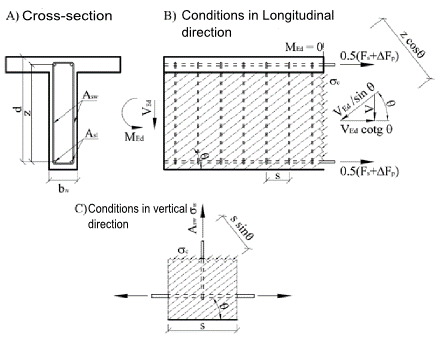
This definition can be clarified so that instead of the centre of gravity of the tensile reinforcement the position of the reinforcement resultant of forces is used. During the development the IDEA RCS program the problem was solved: how to define the effective depth of the cross-section, for which the plane of bending loads doesn’t correspond with the direction of the resultant shear forces. Therefore, the effective depth is defined as the distance of most compressed concrete fibre  to the resultant forces in the tensile reinforcement  (based on bending stress) and in the direction of the resultant shear forces, see Figure 1.17.

Exceptional cases will occur if we are not able to determine the compressed fiber or resultant in the tensile reinforcement. In this case, we recommend using value 0.9 h (90% of section depth in the direction of the resultant shear forces). This value, the user can define in the IDEA RCS program by the setting of code variables.

Lever arm of internal forces

The lever arm of internal forces is in 6.2.3 (3) [2] and is defined as the "distance between tension and compression chords”.  The code does not define how to proceed when  the plane of acting bending moment is different from the direction of resultant shear forces. Therefore, as for the case of the effective depth, we define the distance in the direction of the resultant shear forces. Also here, we can face a similar exception cases, for example, the whole section is under compression, etc. In this case, we take value 0.9 d (90% of the effective section height). This value, the user can set in the IDEA RCS program by the setting of code variables.

Dependence between bending plane inclination and the resultant of shear force is clearly visible in Figure 1.18 and Figure 1.19. With an increase of inclination the values of effective height, lever arms and related resistances are decreasing. The limit state is 90°. For this inclination the lever arm of internal forces cannot be calculated, consequently the lever arm is equal to zero. In this case, the value specified in the setting of code variables is considered. By this, there is a jump at the end of the chart. This study proves the recommended maximum for inclination is about 20°.

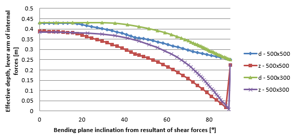
\[ \textsf{\textit{\footnotesize{\qquad Dependence between effective depth, lever arm to the bending plane inclination and the resultant of shear forces.}}}\]

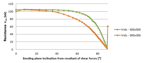
\[ \textsf{\textit{\footnotesize{\qquad Dependence between  resistance Vrds to the bending plane inclination and the resultant of shear.}}}\]

As part of the testing of the RCS application, a study about dependency of shear resistance to changing the normal force was conducted. Resistance V_Rd,max is affected only by the coefficient α_cw, see Fig. 1.20. Fig. 1.21 shows a constant value of resistance V_Rds. For V_Rdc resistance, the decreases cause increasing of normal force. The blue curve in Fig. 1.21 shows the resistance V_Rdc with neglecting the influence of cracks and it was calculated using the formula in section 6.2.2 (1) [2]. Jump in transition between pressure and tension is caused by contributed tensile reinforcement. The red curve is calculated using the formula in section 6.2.2 (2) [2]. After the first crack occurred the dependency curve is same as for 6.2.2 (1) [2].

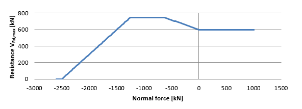
\[ \textsf{\textit{\footnotesize{\qquad Dependency curve of shear resistance VRd,max to normal force.}}}\]

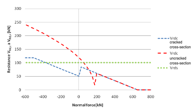
\[ \textsf{\textit{\footnotesize{\qquad Dependency of shear resistances VRd,c a VRd,s to normal force.}}}\]

Torsion

Calculation assumptions

The behavior of a reinforced concrete section subjected to torsion can be divided into two categories - before and after the time when the cracks may first be expected to occur. Before a crack the cross-section behaves as an elastic material. Torsion stress can be expressed by formula   

 \[\tau =~\frac{{{T}_{Ed}}}{{{W}_{t}}}\] 

where W_t je sectional module in torsion.

Cracks in the unreinforced member due to principal tensile torsion stress are also ultimate limit state. The behavior of a reinforced concrete section subjected to torsion can be described on the basis of a thin-walled closed section, see Fig. below. 

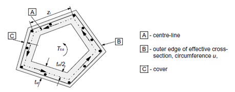
\[ \textsf{\textit{\footnotesize{\qquad Equivalent thin-walled cross-section.}}}\]

Calculation procedure

The process of a reinforced concrete check for torsion is very similar to the check for shear. First of all, we check the concrete resistance. If the concrete check is satisfied, the reinforcement can be designed using the detailing rules. Otherwise, we need to verify the reinforcement and compressive diagonal resistance by calculation.

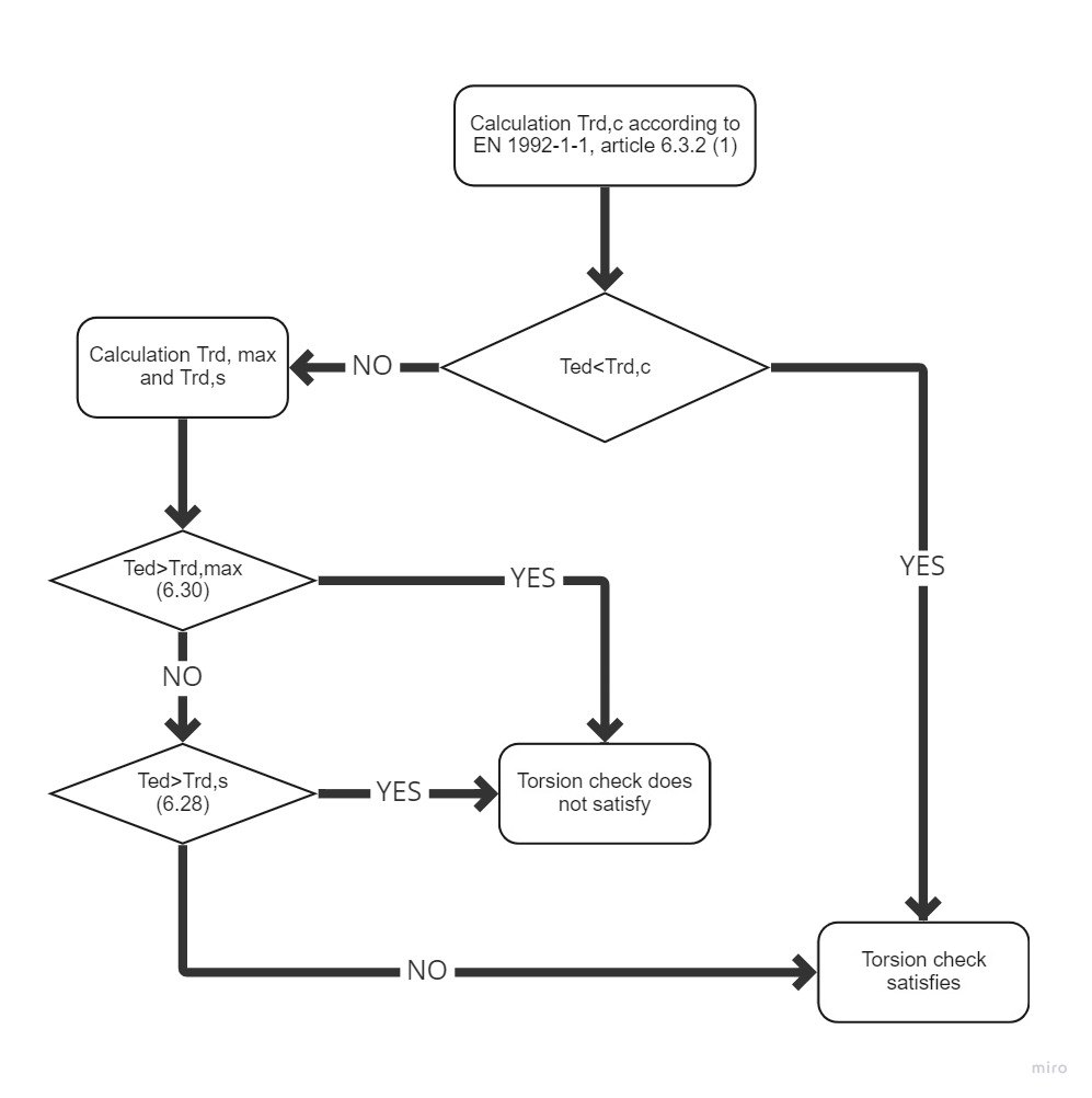
\[ \textsf{\textit{\footnotesize{\qquad Process diagram for torsion check.}}}\]

Resistance

Shear flow in a wall of a thin-walled cross-section under torsion can be expressed as:

\[ {{\tau }_{t}}{{t}_{ef}}=~\frac{{{T}_{Ed}}}{2{{A}_{k}}}\]

Shear force in a wall of a thin-walled cross-section can be expressed as:

\[ V={{\tau }_{t}}{{t}_{ef}}z\]

Where 

τ          Shear flow in wall,

t_ef         is the effective wall thickness,

z           is the side length of wall,

T_Ed       is the torsion moment,

A_k        is the area enclosed by the center-lines of the connecting walls, including inner hollow areas.

Torsion cracking moment, which may be determined by setting f_ctd to previous expression. Thus we get expression for the resistance in torsion without torsion reinforcement.

\[ {{T}_{Rd,c}}=2{{A}_{k}}{{t}_{ef}}{{f}_{ctd}}\]

where  f_ctd       design axial tensile strength of concrete

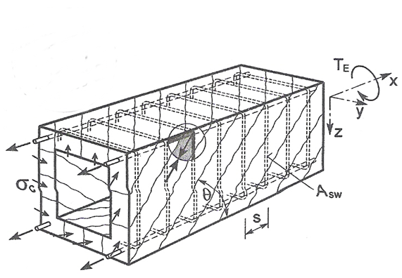
\[ \textsf{\textit{\footnotesize{\qquad Principles of Truss analogy for member under torsion moment.}}}\]

The member resistance with torsion reinforcement is composed from the resistance of compressive concrete diagonals which is based again on the truss analogy method. Compressive stress in the diagonal can be expressed with help of shear force in the wall of a thin-walled cross-section on the wall surface which is in consideration, i.e.

\[{{\sigma }_{c}}=\frac{\frac{{{T}_{Ed}}z}{2{{A}_{k}}\sin \theta }}{z~{{t}_{ef}}\cos \theta }=\frac{{{T}_{Ed}}}{2{{A}_{k}}{{t}_{ef}}\sin \theta \cos \theta }\]

Substitution of  σ_c=σ_cwf_cd and T_Ed=T_Rd,max and expressing of T_Rd,max we get an equation for the compressive diagonal resistance

\[{{T}_{Rd,max}}=2~\nu ~{{\alpha }_{cw}}~{{f}_{cd}}~{{A}_{k}}~{{t}_{ef~\sin \theta ~\cos \theta }}\]

where  

ν          = 0,6 pro f_ck ≤ 60MPa or  for f_ck > 60MPa

α_cw       coefficient which takes account the state of compressive stress in compression chord

f_cd        design value of concrete compressive strength

the shear reinforcement resistance subjected to torsion is again based on stress in the compression diagonal. The stirrup force is equal to the stress in the compressed diagonal on the area which corresponds to the particular stirrup line, i.e.

\[{{A}_{sw}}{{f}_{ywd}}=\frac{{{T}_{Ed}}}{2{{A}_{k}}{{t}_{ef}}\sin \theta \cos \theta }~{{t}_{ef}}~s{{\sin }^{2}}\theta =\frac{{{T}_{Ed}}~s}{2{{A}_{k}}\cot \theta }~\]

Substituting  T_Ed=T_Rd,s and expressing T_Rd,s  we get equation:

 \[{{T}_{Rd,s}}=2{{A}_{k}}\frac{{{A}_{sw}}{{f}_{ywd}}}{s}~\cot \theta\] 

If the longitudinal and shear reinforcement quantity is known, we can define angle θ by the expression

\[{{\tan }^{2}}\theta =\frac{\frac{{{A}_{sw}}{{f}_{ywd}}}{s}}{\frac{{{A}_{sl}}{{f}_{yd}}}{{{u}_{k}}}}\] 

Substitution for T_Rd,s we get

\[{{T}_{Rd,s}}=2{{A}_{k}}\sqrt{\frac{{{A}_{sw}}}{s}{{f}_{ywd~}}\frac{{{A}_{sl}}}{{{u}_{k}}}~{{f}_{yd}}}\]  

Where

A_sw      shear reinforcement area

s           is the radial spacing of stirrups of shear reinforcement

f_ywd      is the effective design strength of the shear reinforcement

A_sl       longitudinal reinforcement area

u_k         is the outer circumference of the cross-section

f_ywd      is the effective design strength of the longitudinal reinforcement

The force in the longitudinal reinforcement can be deducted from The shear force in a wall of a section subject to a pure torsional moment, which is give as:

\[V=\frac{{{T}_{Ed}}}{2{{A}_{k}}}{{u}_{k}}\]

That force is transformed to longitudinal direction and we get:

\[{{F}_{l}}=\frac{{{T}_{Ed}}{{u}_{k}}}{2{{A}_{k}}~\tan \theta }\]

The permitted range of the values for angle θ is similar to the shear check, i.e 1 < cot θ < 2,5. Dependency between resistances can be seen in Fig. below. The diagram shows that with increasing the angle θ  the resistance T_Rd,max is growing,  the resistance T_Rd.s is decreasing and resistance T_Rd,c is constant, since it is not based on the truss analogy method.

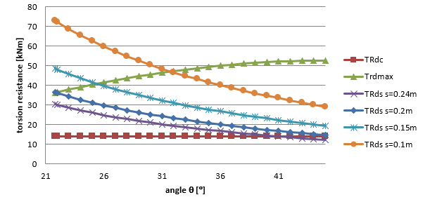
\[ \textsf{\textit{\footnotesize{\qquad Závislost únosnosti průřezu v kroucení na úhlu θ.}}}\]

Calculation of cross-section characteristics for torsion

To check the cross-section for torsion it is necessary to establish a so-called equivalent thin-walled closed section. In determining the dimensions of the equivalent thin-walled cross-section by assuming a rectangular shape. For the true area of rectangular states A = b×h and for the circumference of rectangle u =2 (b +h). Using these two equations can provide alternative thin rectangle-shaped area and periphery of the original cross-section. Solving two equations with two unknowns we get:

\[b=\frac{-u\pm \sqrt{{{u}^{2}}-16A}}{-4}\text{ }\!\!~\!\!\text{ }\]

\[h=\frac{\left( u-2\text{b} \right)}{2}\]

The wall thickness of the effective cross-section can be define from periphery and section area as:

\[t=\text{A}/\text{u}\]

Then the area and periphery defined by center line of the effective cross-section:

\[{{A}_{k}}=\left( \text{h}-\text{t} \right)\text{ }\!\!~\!\!\text{ }\left( \text{b}-\text{t} \right)\text{ }\!\!~\!\!\text{ }\]

\[{{u}_{k}}=2\left( \left( \text{h}-\text{t} \right)+\text{ }\!\!~\!\!\text{ }\left( \text{b}-\text{t} \right) \right)\]

The problem with this method is for cross-section of type T with a wide plate when the overall area and periphery is taken to calculate the dimensions (including this plate). In the future versions of IDEA RCS program, the selection of the most massive cross-section part will be enabled, which will be used to check the torsion.

Interaction

Interaction of shear force and torsion for shear reinforcement

Determination of the force in shear reinforcement due to shear force. 

The calculation is based on the formula for calculating the resistance of the shear reinforcement defined in EN 1992-1-1. Based on equation 6.13 (chap. 6.2.3 (4)) the load-bearing resistance of one stirrup leg can be derived as:

\[{{V}_{Rd,s}}=\frac{{{A}_{sw,V}}}{s}z{{f}_{ywd}}\left( \cot \theta +\cot \alpha  \right)\sin \alpha \cos \beta \]

\[\frac{{{A}_{sw,V}}}{s}={{a}_{sw,V}}\]

A_sw,V .  .  . cross-sectional area of one stirrup leg resisting shear in considered section

s .  .  .  .  . spacing of the shear reinforcement in the direction of the longitudinal member axis 

a_sw,V .  .  . cross-sectional area of the shear reinforcement per unit length

z .  .  .  .  . the inner lever arm. For a member with constant depth, corresponding to the bending moment in the element under consideration. In the shear analysis of reinforced concrete without axial force, the approximate value z = 0,9d may normally be used.

f_ywd .  .  .  the design yield strength of shear reinforcement

θ .  .  .  .  . the angle between the concrete compression strut and the member axis perpendicular to the shear force

α .  .  .  .  . the angle between shear reinforcement and the member axis perpendicular to the shear force

β .  .  .  .  . inclination of the leg of the stirrup relative to the resultant of the applied shearing force

The shear force is redistributed evenly among the individual reinforcement resisting the shear force based on the angle of the reinforcement and the axial stiffness of the individual stirrup legs.

\[{{V}_{ed}}={{V}_{ed,1}}+{{V}_{ed,2}}+...+{{V}_{ed,n}}\]

\[{{V}_{ed}}={{\varepsilon }_{sw,V}}\cdot z\cdot \sum\limits_{i=1}^{{{n}_{V}}}{{{a}_{sw,i,V}}\cdot {{E}_{sw,i,V}}\cdot \left( \cot \theta +\cot {{\alpha }_{i}} \right)\cdot {{\cos }^{2}}{{\beta }_{i}}}\]

Further, the average reinforcement strain considered in the direction of the resultant shear force can be derived:

\[{{\varepsilon }_{sw,V}}=\frac{{{V}_{ed}}}{z\cdot \sum\limits_{i=1}^{{{n}_{V}}}{{{a}_{sw,i,V}}\cdot {{E}_{sw,i,V}}\cdot \left( \cot \theta +\cot {{\alpha }_{i}} \right)\cdot {{\cos }^{2}}{{\beta }_{i}}}}\]

The actual strain of the i-th reinforcement can be calculated as:

\[{{\varepsilon }_{sw,i,V}}=\frac{{{\varepsilon }_{sw,V}}}{\sin {{\alpha }_{i}}}\cdot \cos {{\beta }_{i}}\]

The tension in a given leg of the reinforcement:

\[{{\sigma }_{sw,i,V}}={{\varepsilon }_{sw,i,V}}\cdot {{E}_{si,V}}\]

Determination of the force in individual stirrup due to torsion

The torsional resistance of a section may be calculated on the basis of a thin-walled closed section, in which equilibrium is satisfied by a closed shear flow. Solid sections may be modeled by equivalent thin-walled sections. For non-solid sections, the equivalent wall thickness should not exceed the actual wall thickness.

Shear flow in the walls of a thin-walled closed section due to torsion may be calculated as:

\[{{\tau }_{t}}\cdot {{t}_{ef}}=\frac{{{T}_{ed}}}{2{{A}_{k}}}\]

Shear force in a particular wall is then:

\[{{V}_{i}}={{\tau }_{t}}\cdot {{t}_{ef}}\cdot {{l}_{i}}\]

l_i .  .  .  . length of the centreline of the wall under consideration

Shear force in the web - the length of the web centreline can be substituted by the value of the lever arm "z".

\[{{V}_{ed,T}}=\frac{{{T}_{ed}}}{2{{A}_{k}}}\cdot z\]

Force in stirrups resisting torsion per one meter of the member length (per unit length):

\[{{F}_{sw,T}}=\frac{{{V}_{ed,T}}}{z\cdot \cot \theta }=\frac{{{T}_{ed}}}{2{{A}_{k}}}\cdot tg\theta\]

Decompositions of forces for individual stirrup

If the same material is defined for all stirrups, the resulting stress due to torsion in each stirrup leg is constant. Then:

\[{{\sigma }_{sw,T}}=\frac{{{F}_{sw,T}}}{{{a}_{sw,T}}}\]

where a_sw,T is the total area of stirrups resisting the torsion per unit length.

In the case that individual stirrups have different materials, the axial stiffness of the individual bars must be taken into account.

\[{{F}_{sw,T}}={{F}_{s1,T}}+{{F}_{s2,T}}+{{F}_{s3,T}}+...+{{F}_{sn,T}}=\sum\limits_{i=1}^{{{n}_{T}}}{{{F}_{si,T}}}\]

\[{{\varepsilon }_{sw,T}}=\frac{{{F}_{sw,T}}}{\sum\limits_{i=1}^{{{n}_{T}}}{\left( {{a}_{si,T}}\cdot {{E}_{si,T}} \right)}}\]

n_T .  .  .  . number of legs of reinforcement (groups of reinforcement) resisting torsion

F_si,T .  .  . force in the i-th group of reinforcement resulting from torsion per unit length

a_si,T .  .  . cross-sectional area of the shear reinforcement resisting torsion per unit length 

E_si,T .  .  . Young´s modulus of elasticity of the i-th group of reinforcement resisting torsion

ε_sw,T .  .  strain in the reinforcement due to torsion

The resulting stress in each stirrup due to applied torsion is calculated as:

\[{{\sigma }_{sw,i,T}}={{\varepsilon }_{sw,T}}\cdot {{E}_{si,T}}\]

V+T interaction

The calculation of the stresses in stirrups due to shear and torsion is then a summation of the stresses due to individual load components.  

\[{{\sigma }_{sw,i}}={{\sigma }_{sw,i,V}}+{{\sigma }_{sw,i,T}}\]

Resulting force in the i-th reinforcement:

\[{{F}_{sw,i}}={{a}_{sw,i}}\cdot {{\sigma }_{sw,i}}\]

Interaction of shear, torsion and bending for longitudinal reinforcement

Determination of the force in each longitudinal reinforcement due to the normal force and bending moment

The application RCS is used to calculate the cross-sectional response due to the combination of the normal force and bending moment to determine the stress and strain in the individual longitudinal bars and prestressing reinforcement.

Determination of the force in the individual longitudinal reinforcement due to shear force

The increment of the tensile force in the longitudinal reinforcement ΔF_td from the shear force depends on the geometry of the strut and tie model. 

\[\Delta {{F}_{td}}={{V}_{ed}}\left( \cot \theta -\cot \alpha  \right)\]

ΔF_td .  .  .  increment of tensile force in the longitudinal reinforcement due to the shear force

V_ed .  .  .  . design value of the shear force acting in the section under consideration

θ .  .  .  .  . the angle between the concrete compression strut and the member axis 

α .  .  .  .  . the angle between shear reinforcement and the member axis

For the longitudinal reinforcement located in the tension chord, the resulting force F_t in the longitudinal reinforcement due to the combination N+M+V should be taken not greater than M_Ed,max/z (where M_Ed,max is the maximum moment along the beam)

\[{{F}_{t}}=\frac{{{M}_{Ed}}}{z}+0,5{{V}_{ed}}\left( \cot \theta -\cot \alpha  \right)\le \frac{{{M}_{Ed,\max }}}{z}\]

The force ΔF_td is transmitted by all bonded prestressing tendons and reinforcement located in the part of the cross-section that resists shear (the web in the case of an I-profile). On the safe side, the contribution of prestressing reinforcement can be considered 0. The assumption of the calculation is that the increment of the axial strain of the individual longitudinal reinforcement resisting shear is constant (Δε_s1,V = Δε_s2,V = .... =Δε_p1,V = Δε_p2,V = ... = Δε_V = const.). The derivation is valid for a bilinear reinforcement working diagram with a horizontal plastic branch. In the case of a diagram with an inclined branch, the calculation must be modified.

\[\Delta {{F}_{td}}=\Delta {{F}_{s}}+\Delta {{F}_{s}}\]

\[\Delta {{F}_{td}}=\Delta {{\varepsilon }_{V}}\cdot \sum\limits_{i=1}^{{{n}_{s,V}}}{{{A}_{sl,i,V}}\cdot {{E}_{sl,i,V}}}+\Delta {{\varepsilon }_{V}}\cdot \sum\limits_{i=1}^{{{n}_{p,V}}}{{{A}_{pl,i,V}}\cdot {{E}_{pl,i,V}}}\]

Δε_V .  .  .  . strain increment in the longitudinal reinforcement due to the shear force

n_s,V .  .  .  . number of longitudinal reinforcements resisting the shear force

A_sl,i,V .  .  . area of the i-th longitudinal reinforcement resisting the shear force

E_sl,i,V .  .  . Young´s modulus of elasticity of the i-th longitudinal reinforcement resisting the shear force

n_p,V .  .  .  . number of tendons resisting the shear force

A_pl,i,V .  .  . area of the i-th tendon resisting the shear force

E_pl,i,V .  .  . Young´s modulus of elasticity of the i-th tendon resisting the shear force

After determining the value of force ΔF_td, the average reinforcement strain Δε_V can then be calculated.

\[\Delta {{\varepsilon }_{V}}=\frac{\Delta {{F}_{td}}}{\sum\limits_{i=1}^{{{n}_{s,V}}}{{{A}_{sl,i,V}}\cdot {{E}_{sl,i,V}}}+\sum\limits_{i=1}^{{{n}_{p,V}}}{{{A}_{pl,i,V}}\cdot {{E}_{pl,i,V}}}}\]

Stress increment in the individual longitudinal bars due to the applied shear force:

for rebar \[\Delta {{\sigma }_{sl,i,V}}=\Delta {{\varepsilon }_{V}}\cdot {{E}_{sl,i,V}}\]

for tendon \[\Delta {{\sigma }_{pl,i,V}}=\Delta {{\varepsilon }_{V}}\cdot {{E}_{pl,i,V}}\]

Determination of the force in each longitudinal reinforcement from torsion

It is very important to determine the longitudinal reinforcement that resist the torsion. These are the reinforcement that are located in a torsion-resisting alternate effective thin-walled cross-section.

\[\frac{\sum{{{A}_{sl}}{{f}_{yd}}}}{{{u}_{k}}}=\frac{{{T}_{ed}}}{2{{A}_{k}}}\cot \theta \]

According to EN 1992-1-1, several conditions must be fulfilled for longitudinal torsion resistant reinforcement:

- the reinforcement should be uniformly distributed along the length z_i, but in small cross-sections the reinforcement may be concentrated at the corners of the stirrup

- the maximum axial distance of the longitudinal reinforcement is 350 mm

The contribution of prestressing reinforcement is not considered according to EN 1992-1-1.

The code EN 1992-2 states that the contribution of prestressing reinforcement may be considered, but the maximum stress increment in the prestressing reinforcement shall not exceed Δσ_p ≤ 500MPa. Then the formula can be modified:

\[\frac{\sum{{{A}_{sl}}{{f}_{yd}}+\sum{{{A}_{p}}\Delta {{\sigma }_{p}}}}}{{{u}_{k}}}=\frac{{{T}_{ed}}}{2{{A}_{k}}}\cot \theta\]

However, since the increment of prestressing reinforcement can be considered, but it is at the user's choice. Currently, prestressing reinforcement is not considered in the calculation. 

The assumption of the calculation is that the increment of the axial strain of each longitudinal shear resisting reinforcement is constant (Δε_s1,T = Δε_s2,T = .... =Δε_p1,T = Δε_p2,T = ... = Δε_T = const.). The derivation is valid for a bilinear reinforcement working diagram with a horizontal plastic branch. In the case of a diagram with an increasing branch, the calculation must be modified.

\[\frac{\sum\limits_{i=1}^{{{n}_{T}}}{{{A}_{sl,i,T}}\cdot \Delta {{\sigma }_{s,i,T}}}}{{{u}_{k}}}=\frac{{{T}_{ed}}}{2{{A}_{k}}}\cot \theta\]

\[\frac{\sum\limits_{i=1}^{{{n}_{T}}}{{{A}_{sl,i,T}}\cdot \Delta {{\varepsilon }_{T}}\cdot {{E}_{s,i,T}}}}{{{u}_{k}}}=\frac{{{T}_{ed}}}{2{{A}_{k}}}\cot \theta\]

\[\Delta {{\varepsilon }_{T}}=\frac{{{T}_{ed}}\cdot {{u}_{k}}}{2{{A}_{k}}\cdot \sum\limits_{i=1}^{{{n}_{T}}}{{{A}_{sl,i,T}}\cdot {{E}_{s,i,T}}}}\cot \theta\]

\[\frac{\sum\limits_{i=1}^{{{n}_{T}}}{{{A}_{sl,i,T}}\cdot \Delta {{\sigma }_{s,i,T}}}}{{{u}_{k}}}=\frac{{{T}_{ed}}}{2{{A}_{k}}}\cot \theta\]

\[\frac{\sum\limits_{i=1}^{{{n}_{T}}}{{{A}_{sl,i,T}}\cdot \Delta {{\varepsilon }_{T}}\cdot {{E}_{s,i,T}}}}{{{u}_{k}}}=\frac{{{T}_{ed}}}{2{{A}_{k}}}\cot \theta\]

\[\Delta {{\varepsilon }_{T}}=\frac{{{T}_{ed}}\cdot {{u}_{k}}}{2{{A}_{k}}\cdot \sum\limits_{i=1}^{{{n}_{T}}}{{{A}_{sl,i,T}}\cdot {{E}_{s,i,T}}}}\cot \theta\]

T_ed .  .  .  . the design value of the torque applied in the section under consideration

θ .  .  .  .  . inclination of the compression diagonals with respect to the longitudinal axis of the beam (identical to that for the shear force)

u_k .  .  .  .  perimeter of the area A_k

A_f .  .  .  .  the area defined by the centreline of the replacement hollow thin-walled section

n_s,T .  .  .  .number of longitudinal concrete reinforcement resisting torque

A_sl,i,T .  .  . area of the i-th longitudinal concrete reinforcement resisting torque

Δε_T .  .  .  .the change in the longitudinal reinforcement transformation due to the torque

Δσ_s,i,T .  .  change in stress in the i-th longitudinal reinforcement due to torque

E_sl,i,T .  .  . modulus of elasticity of the i-th longitudinal concrete reinforcement resisting the torque

Stress increment in each longitudinal reinforcement from the applied torque:

\[\Delta {{\sigma }_{sl,i,T}}=\Delta {{\varepsilon }_{T}}\cdot {{E}_{sl,i,T}}\]

Stress limitation check

The check is based on general assumptions, where two states of the cross-section are resolved: the uncracked section (the tensile strength of the concrete is not ignored) and the fully cracked section (the tensile strength of the concrete is ignored). The solution with ignored concrete tensile strength is considered under the assumptions of Article 7.1 (2) EN 1992-1-1.

When calculating the stress and deflections it is considered as an uncracked section, if the tensile stress in bending does not exceed f_ct, eff. The value of f_ct, eff can be considered as f_ctm or f_ctm,fl. The f_ctm value is used when calculating the crack width and tensile stiffening.

As part of this check, we deal with four basic cases in terms of stress limit.

• 7.2 (2) Compressive stress in members exposed to environments of exposure classes XD, XF and XS should be limited:

\[\left| {{s}_{c}} \right|\le {{k}_{1}}{{f}_{ck}}\]

\[{{k}_{1}}=0,6\]

• 7.2 (3) The stress in the concrete under the quasi-permanent loads is limited:

\[\left| {{s}_{c}} \right|\le {{k}_{2}}{{f}_{ck}}\]

\[{{k}_{2}}=0,45\]

• 7.2 (5) Tensile stresses in the reinforcement under the characteristic combination of loads shall be limited:

\[\left| {{s}_{s}} \right|\le {{k}_{3}}{{f}_{yk}}\]

\[{{k}_{3}}=0,8\]

• 7.2 (5) Where the stress is caused by an imposed deformation, the tensile stress should not exceed:

\[\left| {{s}_{s}} \right|\le {{k}_{4}}{{f}_{yk}}\]

\[{{k}_{4}}=1\]

Where values k₁, k₂, k₃, k₄ for use in a Country may be found in its National Annex. The recommended values are 0,8; 1 and 0,75 respectively, characteristic yield stress of the reinforcement, f_ck characteristic cylinder strength f_ck determined at 28 days.

Cracks

The formation of cracks

A characteristic feature of reinforced concrete structures under bending or tensile stress is the occurrence of cracking failure at points where the tensile stress in the concrete exceeds the tensile strength of the concrete. For the durability of the structure and also for the aesthetics of the structure, it is important to ensure that the resulting cracks are as small as possible. The calculation of the crack widths as well as the maximum widths allowed for the different exposure classes are given in EN 1992-1-1, Chapter 7.3.

In the first step of the calculation, it is determined whether the cross-section is cracked or not. The crack width itself is always calculated from the quasi-permanent or frequent load combination (depending on the national annex), but the crack formation has to be checked from all specified SLS combinations. Thus, two cases can occur:

• The maximum tensile stress in the concrete fibers will not exceed the tensile strength of the concrete from any load combination (quasi-permanent M_E,qp, frequent M_E,fr, or characteristic M_E,k), and hence we consider the cross-section without cracks.

\[{{M}_{E,i}}\le {{M}_{cr}}={{f}_{ct,ef}}\frac{{I}_{I}}{h-{{a}_{I}}}\]

• If cracks develop for any of the combinations (quasi-permanent, frequent, or characteristic), i.e. the bending moment developed from the considered load combination is greater than the critical moment M_cr, the cross-section is cracked from that load combination, and the characteristics of the cracked cross-section and the crack width have to be calculated.

\[{{M}_{E,i}}>{{M}_{cr}}={{f}_{ct,ef}}\frac{{I}_{I}}{h-{{a}_{I}}}\]

M_E,i   .   .   the bending moment obtained from some SLS load comb. Thus, it can be M_E,qp, M_E,fr, or M_E,k. 

f_ct,ef   .   .  the tensile strength of the concrete at the considered time. If the concrete is older than 28 days, we consider a strength equal to f_ctm.

Crack width calculation

In a bending-loaded element, the crack formation is divided into 2 phenomena:

• Crack formation phase (stage number 2 in Fig. 1)
• Stabilized crack development (stage number 3 in Fig. 1)

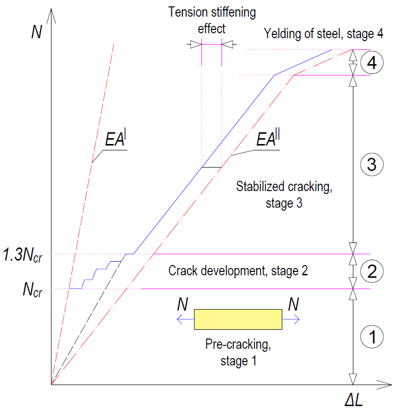
\[ \textsf{\textit{\footnotesize{Fig. 1  Stages of the behavior of the reinforced concrete cross-section during loading}}}\]

Crack development stage

This is the initial part of the process when individual cracks are still gradually appearing until the entire tensile part of the member is affected by cracks that are approximately equally distributed along the length of the member. The first crack is formed when the force in the tensioned strip exceeds the value of the critical force N_r (Critical tensile force, see below), and further cracks develop up to a level of load exerting a force in the tensioned strip equal to approximately 1.3N_cr (phase number 2 in Fig. 1).

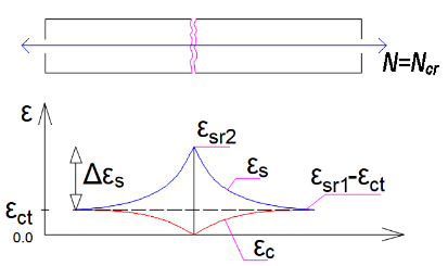
\[ \textsf{\textit{\footnotesize{Fig. 2  Strains of concrete and reinforcement at the moment of the first crack}}}\]

The developing cracks are divided into 2 types - primary and secondary cracks. Primary cracks occur in the tensile fibers when the effective tensile strength of the concrete (f_ct,eff) is reached. Primary cracks represent the first pattern of cracks (Fig. 2). Shorter secondary cracks are then formed between the primary cracks (Fig. 3). At stresses corresponding to about 1.2 to 1.5 σ_sr (usually a mean value of 1.3 σ_sr is considered, where σ_sr is the stress in the reinforcement at the formation of primary cracks in the tensile zone of the concrete), the development of secondary cracks is also completed.

\[ \textsf{\textit{\footnotesize{Fig. 3  Primary and secondary cracks}}}\]

The crack width at the crack formation stage can be calculated as follows:

\[{{w}_{k}}=2{{l}_{s,\max }}\left( {{\varepsilon }_{sm}}-{{\varepsilon }_{cm}} \right)\]

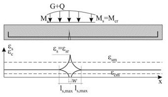
\[ \textsf{\textit{\footnotesize{Fig. 4  Characteristics of the transmission length for the first crack}}}\]

Stabilized cracking stage

After exceeding approximately 1.3 times the critical force in the tensile zone, no new cracks are formed, the number of cracks in the element is stabilized, and only the width of the existing cracks increase with further loading (stage number 3 in Fig. 1).

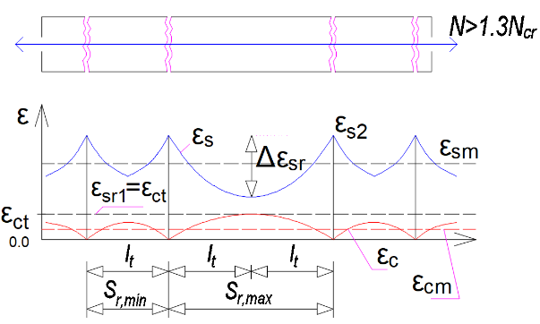
\[ \textsf{\textit{\footnotesize{Fig. 5  Strains of concrete and reinforcement at the stabilized cracking stage}}}\]

The crack width during stable development can be calculated as:

\[{{w}_{k}}={{s}_{r,\max }}\left( {{\varepsilon }_{sm}}-{{\varepsilon }_{cm}} \right)\]

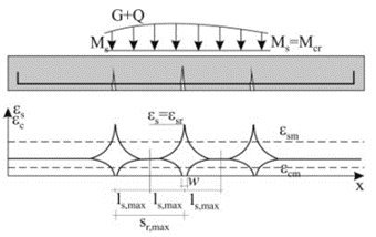
\[ \textsf{\textit{\footnotesize{Fig. 6  Stabilized cracking}}}\]

Critical tensile force

The calculation is based on the Tension Chord Model (TCM). The basic consideration is to calculate the ultimate capacity of a reinforced concrete strip formed by a reinforcing bar of area A_s,eff surrounded by an effective area of tensile concrete A_c,eff, which is able to resist the tensile stress until the tensile strength f_ct,eff is exceeded (normally we consider f_ctm). Assuming a perfect bond between the reinforcement and the concrete, we can consider that until the first crack occurs, the remodeling of the reinforcement and the surrounding concrete is identical. Then the maximum force in the tensile strip just before the first crack N_r can be determined:

\[{{N}_{r}}={{A}_{c,eff}}\cdot {{f}_{ctm}}+{{A}_{s,eff}}\cdot {{\sigma }_{s}}\]

By introducing the substitution

\[{{\alpha }_{e}}={}^{{{E}_{s}}}/{}_{{{E}_{cm}}};{{\rho }_{p,eff}}={}^{{{A}_{s,eff}}}/{}_{{{A}_{c,eff}}}\]

we get:

\[{{N}_{r}}={{A}_{c,eff}}\cdot {{f}_{ctm}}\cdot \left( 1+{{\alpha }_{e}}\cdot {{\rho }_{p,eff}} \right)\]

Just after the formation of the first crack, the entire force N_r is transferred by the reinforcement and thus the stress in the reinforcement passing through the just-formed crack can be calculated as:

\[{{\sigma }_{sr}}=\frac{{{f}_{ctm}}}{{{\rho }_{p,eff}}}\cdot \left( 1+{{\alpha }_{e}}\cdot {{\rho }_{p,eff}} \right)\Rightarrow {{\varepsilon }_{sr}}=\frac{{{f}_{ctm}}}{{{E}_{s}}\cdot {{\rho }_{p,eff}}}\cdot \left( 1+{{\alpha }_{e}}\cdot {{\rho }_{p,eff}} \right)\]

Crack width calculation according to EC 1992-1-1

The following equation is used to calculate the width of cracks on reinforced concrete elements:

\[{{w}_{k}}={{s}_{r,\max }}\left( {{\varepsilon }_{sm}}-{{\varepsilon }_{cm}} \right)\]

s_r,max   .   .   .   maximum crack spacing

ε_sm  .   .   .   .   the average strain of the reinforcement from the load combination, including the effects of tension stiffening.

ε_cm  .   .   .   .   average strain of concrete between cracks

Calculation of the strain difference

The difference in the strain of reinforcement and concrete between cracks can be obtained from the equation:

\[{{\varepsilon }_{sm}}-{{\varepsilon }_{cm}}=\frac{{{\sigma }_{s}}-{{k}_{t}}\cdot \frac{{{f}_{ct,eff}}}{{{\rho }_{p,eff}}}\cdot \left( 1+{{\alpha }_{e}}\cdot {{\rho }_{p,eff}} \right)\,}{{{E}_{s}}}\ge 0,6\frac{{{\sigma }_{s}}}{{{E}_{s}}}\]

σ_s      .   .   .   .   the stress in the reinforcement in the crack from the load combination under consideration

k_t      .   .   .   .   an empirical coefficient taking into account the average strain, depended on the duration of the load. It can take values of 0.6 for short-term analysis. For the long-term analysis, the reduction of the stiffness of the composite to about 70% is taken into account, so its value is 0.4, which includes the rate of degradation of the cohesion between the reinforcement and the concrete due to time.

α_e     .   .   .   . the effective ratio of elastic moduli

\[{{\alpha }_{e}}={}^{{{E}_{s}}}/{}_{{{E}_{cm}}}\]

ς_p,_eff  .   .   .   .   effective level of reinforcement

\[{{\rho }_{p,eff}}={}^{\left( {{A}_{s,eff}}+{{\xi }^{2}_{1}}A_{p}^{\acute{\ }} \right)}/{}_{{{A}_{c,eff}}}\]

A_c,_eff .   .   .   .   the effective area of the concrete in tension surrounding the reinforcement (determination of A_c,eff below)

A_s,_eff .   .   .   .   the area of bonded reinforcement located in the area of A_c,_eff

A_p´    .   .   .   .   is the area of pre- or post-tensioned tendons within A_c,_eff

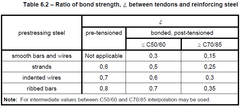
ξ₁  .   .   .   .   .   is the adjusted ratio of bond strength, taking into account the different diameters of prestressing and reinforcing steel:

\[{{\xi }_{1}}=\sqrt{\xi \,\cdot \,\frac{{{\phi }_{s}}}{{{\phi }_{p}}}}\]

ξ  .   .   . the ratio of bond strength of prestressing and reinforcing steel (Table 6.2)

ϕ_s   .   .  largest bar diameter of reinforcing steel

ϕ_p   .   .  the diameter or equivalent diameter of prestressing steel

For bundles, A_p is the area of reinforcement in the tendon

\[{{\phi }_{p}}=1,6\sqrt{{{A}_{p}}}\]

For single seven-wire strands where φ_wire is the wire diameter

\[{{\phi }_{p}}=1,75\,\,{{\phi }_{wire}}\]

For single three-wire strands where φ_wire is the wire diameter

\[{{\phi }_{p}}=1,20\,\,{{\phi }_{wire}}\]

If only prestressing reinforcement is used to prevent cracking, then the following must be considered.

\[{{\xi }_{1}}=\sqrt{\xi \,}\]

In prestressed members, a minimum area of bonded reinforcement is not required as long as, under the characteristic combination of loading and the characteristic value of prestressing force the tensile stress in any fiber is not greater than the tensile strength of the concrete, f_ct,eff. (see EN 1992-1-1 ch. 7.3.2 for more details)

The effective area of concrete in tension

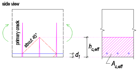
An important but simultaneously the most complicated step of the calculation is determining the effective area of the tensile concrete surrounding the reinforcement. Both the Eurocode and the Model Code consider simple modes of loading, where the reinforced concrete element is loaded by uniaxial bending or tension. The value of the effective height is determined as:

\[{{h}_{c,eff}}=\min \left\{ 2,5\left( h-d \right);\frac{\left( h-x \right)}{3};{}^{h}/{}_{2} \right\}\]

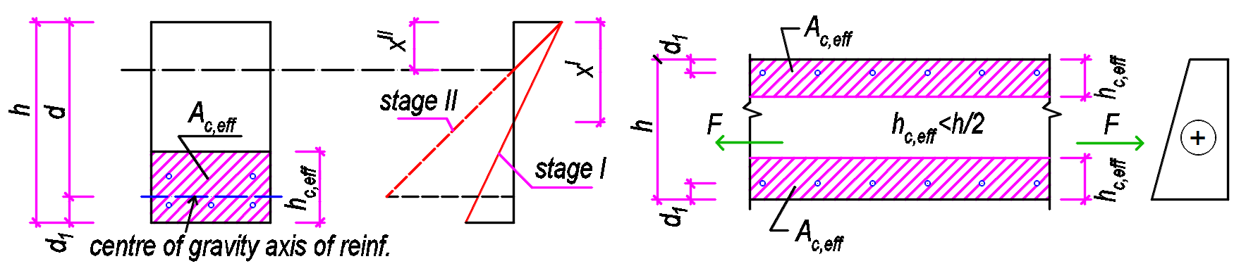
\[ \textsf{\textit{\footnotesize{Fig. 6  Determination of Ac,eff for bent members (left) and members in tension (right)}}}\]

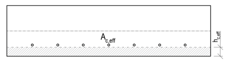
Usually, the value h_c,eff = 2,5(h-d) is critical. For tensioned elements, the upper limit is h/2, while for bent elements it is (h-x)/3. However, the area A_c,eff is also limited by the width determined from equation 5(c+ϕ/2). If the spacing of the reinforcements is greater than 5(c+ϕ/2), then the effective area of the tensioned concrete of width 5(c+ϕ/2) is considered for the individual bars.

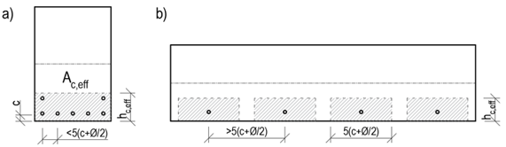
\[ \textsf{\textit{\footnotesize{Fig. 9  Determination of Ac,eff based on reinforcement spacing}}}\]

Maximum crack distance

When calculating the maximum crack distance s_r,max, two cases can occur:

• The axial distance of the bonded reinforcement does not exceed a distance of 5(c+ϕ/2) - Fig. 9a
• The axial distance of the bonded reinforcements is greater than 5(c+ϕ/2) - Fig. 9b

The calculation of the maximum crack distance s_r,max for the case that the axial distances of the reinforcements do not exceed the value 5(c+ϕ/2) is defined as follows:

\[{{s}_{r,\max }}={{k}_{3}}c+{{k}_{1}}{{k}_{2}}{{k}_{4}}\frac{\phi }{{{\rho }_{p,eff}}}\]

c  .    .   .   .   .   concrete cover value in mm. Since the cover value may be different for the edge reinforcement to both the horizontal and vertical edges, it is recommended to consider the maximum cover value found for the reinforcement under consideration.

ϕ     .   .   .   .   diameter of the bonded reinforcement. In the case of different reinforcement diameters, the equivalent diameter shall be calculated in accordance with EN 1992-1-1 Equation 7.12.

\[{{\phi }_{eq}}=\frac{{{n}_{1}}\phi _{1}^{2}+{{n}_{2}}\phi _{2}^{2}}{{{n}_{1}}{{\phi }_{1}}+{{n}_{2}}{{\phi }_{2}}}\]

k₁ .   .   .   . is a coefficient that takes account of the bond properties of the bonded reinforcement

• k₁ = 0,8 for high bond bars
• k₁ = 1,6 for bars with an effectively plain surface (e.g. prestressing tendons)

k₂ .   .   .   . is a coefficient that takes account of the distribution of strain

• k₂ = 1,0 for bending
• k₂ = 0,5 for pure tension

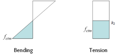
For cases of eccentric tension or for local areas, intermediate values of k₂ should be used which may be calculated from the relation:

\[{{k}_{2}}=\frac{{{\varepsilon }_{1}}+{{\varepsilon }_{2}}}{2{{\varepsilon }_{1}}}\]

k₃      .   .   .   .  coefficient expressing the length of the area close to a crack where the bond between the concrete and the reinforcement is broken. The recommended value of the basic EC k₃ = 3,4 may be modified by the National Annex. 

k₄      .   .   .   .   coefficient expresses the relationship between the bond and tensile strength of concrete. The recommended value of the basic EC k4 = 0.425 may be adjusted by the National Annex.

The calculation of the maximum crack distance s_r,max for the case that the axial distances of the reinforcements exceed the value 5(c+ϕ/2) is defined as follows:

\[{{s}_{r,\max }}=1,3\left( h-x \right)\]

Maximum crack distance values according to the equation

\[{{s}_{r,\max }}=1,3\left( h-x \right)\]

should always be greater than the values determined by the equation

\[{{s}_{r,\max }}={{k}_{3}}c+{{k}_{1}}{{k}_{2}}{{k}_{4}}{\phi }/{{{\rho }_{p,eff}}}\;\]

otherwise, it is recommended to consider the larger distance obtained from the above equations. The equation for the strain in the concrete/reinforcement is not modified for the case of the large axial distance of the reinforcement. In areas with controlled crack widths, the axial distance of individual reinforcements should not be greater than 5(c+ϕ/2).

Crack width calculation implemented in RCS

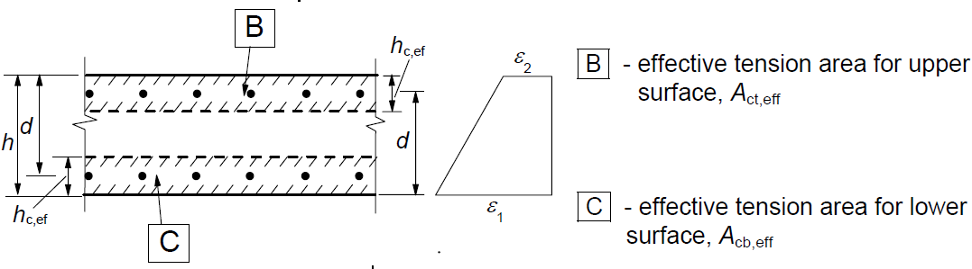
Determination of effective area A_c,eff

Because it is not so straightforward to determine which reinforcement can be considered as longitudinal crack-resisting reinforcement, A_c,eff is determined by using the following iterative process.

• Of all the reinforcement acting in tension, the tensile force center C_g,s,1 is determined. The effective depth of the reinforcement d is the distance between C_g,s, and the most compressed concrete fiber calculated in the direction of the resultant bending moment. At the same time, the position of the neutral axis and the height of the compressed area x for the cracked cross-section are determined. This makes it possible to determine the effective height h_c,eff:

\[{{h}_{c,eff}}=\min \left\{ 2,5\left( h-d \right);\frac{\left( h-x \right)}{3};{}^{h}/{}_{2} \right\}\]

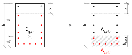
• By excluding all reinforcement that lie outside the A_c,eff,1, the new center of the reinforcement C_g,s,2 is determined, together with the new effective depth of the reinforcement d, effective height h_c,eff is determined in the same way as in the previous step, only with changed input values.

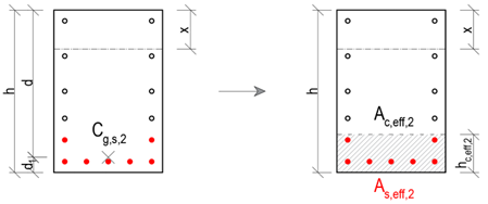
Again, it is checked that all the tensioned reinforcement under consideration lies in the A_c,eff,2. If this condition is satisfied, the iteration can be terminated and the values of h_c,eff,2, A_c,eff,2 and A_s,eff,2 are displayed as the resulting values in IDEA StatiCa RCS.

Possible cases of crack width calculation

In general, three cases can occur when calculating crack widths:

• The tensile reinforcement lies in the region A_c,eff, with the axial distance of the individual reinforcements being less than 5(c+ϕ/2). Then the following definitions are used for the calculation:

\[{{s}_{r,\max }}={{k}_{3}}c+{{k}_{1}}{{k}_{2}}{{k}_{4}}\frac{\phi }{{{\rho }_{p,eff}}}\]

\[{{\varepsilon }_{sm}}-{{\varepsilon }_{cm}}=\frac{{{\sigma }_{s}}-{{k}_{t}}\,\cdot \,\frac{{{f}_{ct,eff}}}{{{\rho }_{p,eff}}}\,\cdot \,\left( 1+\,{{\alpha }_{e}}\cdot \,{{\rho }_{p,eff}} \right)\,\,}{{{E}_{s}}}\ge 0,6\frac{{{\sigma }_{s}}}{{{E}_{s}}}\]

• The tensile reinforcement lies in the A_c,eff, with the axial distance of the individual reinforcements exceeding the distance 5(c+ϕ/2). Then the following definitions are used for the calculation:

\[{{s}_{r,\max }}=1,3\left( h-x \right)\]

\[{{\varepsilon }_{sm}}-{{\varepsilon }_{cm}}=\frac{{{\sigma }_{s}}-{{k}_{t}}\,\cdot \,\frac{{{f}_{ct,eff}}}{{{\rho }_{p,eff}}}\,\cdot \,\left( 1+\,{{\alpha }_{e}}\cdot \,{{\rho }_{p,eff}} \right)\,\,}{{{E}_{s}}}\ge 0,6\frac{{{\sigma }_{s}}}{{{E}_{s}}}\]

• The tensile reinforcement does not lie in the A_c,eff (this may be caused, for example, by thick cover). 

In this case it would not be possible to calculate the width of the cracks. Therefore, the calculation of the effective height h_c,eff is modified as follows:

\[{{h}_{c,eff}}=\min \left\{ 2,5\left( h-d \right);h/2 \right\}\]

At the same time, the following nonconformity is displayed:

The effective concrete area in tension surrounding the reinforcement or prestressing tendons of depth h_c,eff, where h_c,eff is the lesser of 2.5(h – d) or h/2. Considering value as (h – x)/3, the reinforcement is out of the effective area of concrete in tension, and therefore it would not be possible to calculate crack width according to clause 7.3.4.

N-M-κ diagram

The N-M-κ diagram shows an element's curvature (bending stiffness) as a function of an applied bending moment and normal force. There are three types of N-M-κ diagrams:
- short-term,
- long-term
- ULS.
These diagrams differ in the types of stress-strain diagrams used for the calculation (explained below).

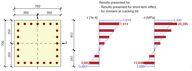
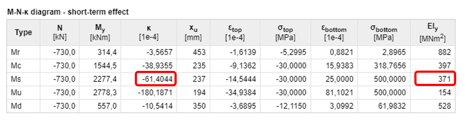
The stiffness calculation for selected characteristic states of the cross-section is used to determine the N-M-κ diagram. In general, it can be any cross-sectional state from which the response is calculated and from which the bending stiffness and curvature are derived. In IDEA RCS, we consider four characteristic points (M_r, M_c, M_s and M_u)

M_r - the cracking moment 

The cross-section is subjected to user-defined normal force and the plane of strain starts to rotate (in the direction of the specified bending moment) until the ultimate tensile strength of the concrete is reached in a concrete fibre (for concrete grade C30/37 this is f_ctm = 2,896 MPa). A bilinear stress-strain diagram with a horizontal plastic branch for both reinforcement and concrete is used for the calculation.

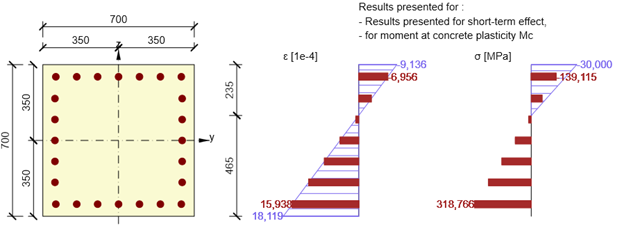
M_c - the bending moment when the compressive strength of the concrete is reached

From the previous step, the most utilized concrete fibre in compression is identified. For this fibre, the strain at the ultimate strength of concrete (f_ck/E_cm for short-term, f_ck/E_ceff for long-term and f_cd/E_cm for the ULS diagram) is set. Based on the defined normal force and the direction of bending moment, the iteration process to find the plane of strain is run to find an equilibrium between the response of the cross-section and the defined normal force.  A bilinear stress-strain diagram with a horizontal plastic branch for both reinforcement and concrete is used for the calculation.

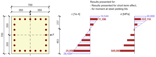
M_s - the bending moment when the yield strength in the most utilized reinforcement bar is reached

Another characteristic point of the N-M-κ diagram is the stress-state of the cross-section when the yield strength in the most utilized reinforcement bar is reached (rebar strain is equal to f_yk/E_s for the short- and long-term diagrams, f_yd/E_s for the ULS diagram). The iteration process finds an equilibrium of normal forces in the cross-section by rotating the plane of strain around the point specified by the position of the most utilized reinforcement bar. A bilinear stress-strain diagram with a horizontal plastic branch for both reinforcement and concrete is used for the calculation.

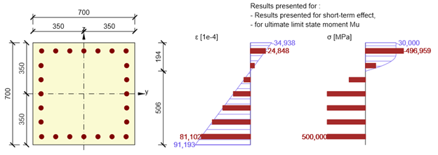
M_u - the bending moment at the ultimate limit state

This is the ultimate load bearing capacity of a cross-section in bending, when the cross-section is subjected to defined design normal force N_ed. For the calculation of the cross-sectional capacity it is assumed that the compressive strength in the most utilized fibre of concrete and the tensile strength in most utilized reinforcement bar are reached (maximum strain for concrete ε_cu = 0,1 and for reinforcement ε_s,max = 0,5. A bilinear stress-strain diagram with a horizontal plastic branch for the reinforcement and a parabola-rectangular diagram for the concrete are used for the calculation.

The resulting stiffness and curvature due to the user-defined combination of normal force and bending moment ( Md) are then calculated using linear interpolation of the individual characteristic points of the N-M-κ diagram.

Calculation of stiffnesses and curvatures

The stiffnesses and curvatures for each cross-sectional stress state (M_r, M_c, M_s or M_u)are calculated directly from the rotation of the plane of strain. 

\[E{{A}_{x}}=\frac{N}{{{\varepsilon }_{x}}}\]

E_Ax .   .    axial stiffness of the element

N . .   .   . the specified normal force

ε_x .   .   .  axial strain at the centre of gravity of the concrete cross-section

\[E{{I}_{y}}=\frac{M}{\kappa }\]

E_Iy .   .   .   bending stiffness of the element

M .   .   .    the calculated bending moment M_r, M_c, M_s or M_u

κ .   .   .   . the curvature of the element, calculated as the tangent of the angle between the plane of the strain and the longitudinal element axis

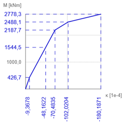
Practical example

A concrete cross-section (concrete grade C30/37) is reinforced with ϕ32 reinforcement (grade B500B). The defined quasi-permanent combination is N = -730 kN and M_y = 557 kNm.

The plane of strain for the characteristic point M_s is determined by IDEA RCS as follows:

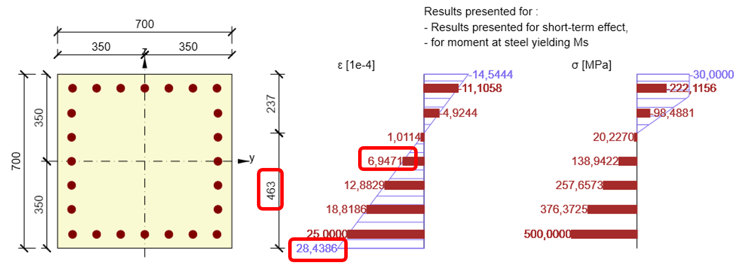
\[E{{A}_{x}}=\frac{N}{{{\varepsilon }_{x}}}=\frac{730}{6,9471\cdot {{10}^{-4}}}=1050,798MN\]

\[\kappa =\frac{28,4386\cdot {{10}^{-4}}}{0,463}=61,422\cdot {{10}^{-4}}{{m}^{-1}}\]

\[E{{I}_{y}}=\frac{{{M}_{s}}}{\kappa }=\frac{2277,4}{61,422\cdot {{10}^{-4}}}=370,776MN{{m}^{2}}\]

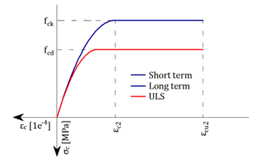
Stress-strain diagrams used for the calculation

Reinforcement - M_r, M_c, M_s and M_u

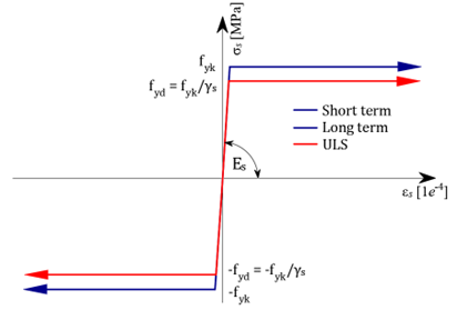
Concrete - M_r, M_c, M_s

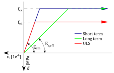
Concrete - M_u

Literature

[1] Bradáč Betonové konstrukce (concrete structures), 1.part: Dimensioning of members from reinforced and plainconcrete, EXPERT Ostrava, 1996

[2] ČSN EN 1992-1-1 (73 1201) Eurocode 2: Design of concrete structures - Part 1-1: General rules and rules for buildings, inc. change NA ed. A (2007) and revision 1 (2009)

[3] ČSN EN 1992-2 (73 6208) Eurokód 2: Navrhování betonových konstrukcí - Část 2: Betonové mosty - Navrhování a konstrukční zásady

[4] Navrátil, J. Předpjaté betonové konstrukce. 2. vydání, Akademické nakladatelství CERM, Vysoké učení technické v Brně, Fakulta stavební, 2008

[5] Šmiřák, S. Pružnost a plasticita I, Vysoké učení technické v Brně, Akademické nakladatelství CERM, Brno, 1999

[6] Vondráček, R. Numerical Methods in Nonlinear Concrete Design, Diplomová práce, ČVUT, Praha, 2000

[7] Zich, M. a kolektiv Konstrukční Eurokódy - Příklady posouzení betonových prvků dle Eurokódů, on-line book http://www.stavebniklub.cz/konstrukcni-eurokody-onbecd/, Verlag Dashöfer, 2010