Structural design of concrete 3D discontinuities in IDEA StatiCa Detail (BETA)

Introduction to the 3D CSFM method

General introduction for the structural design of concrete 3D details
Main assumptions and limitations
Mohr-Coulomb plasticity theory implementation in 3D CSFM
General mechanics assumptions for 3D CSFM

Analysis model of IDEA StatiCa 3D Detail

Introduction to finite element implementation
Finite element types
Meshing in 3D CSFM
Solution method and load-control algorithm for 3D CSFM
Presentation of 3D results

Model verification

Limit states

Structural element checks according to Eurocode

Material models in 3D CSFM
Partial safety factors
Ultimate limit state checks

Introduction to the 3D CSFM method

A general introduction to the structural design of concrete 3D details

In practice, engineers may encounter different types of finite elements (from simple 1D bar elements to more complicated 3D brick elements) that are used in a variety of applications for the analysis and design of structural elements. A common feature of most of the computations in practice tends to be the linear behavior of the models, the advantages of which are undoubtedly speed, clarity, and simply the fact that for a large variety of problems, this solution is quite sufficient.

Especially in the world of concrete structures, it often happens that the linear approach is not sufficient simply because after the first cracks appear in the loaded element, the stresses are redistributed and the problem becomes significantly non-linear.

For these cases, it is necessary to choose one of the more sophisticated approaches. For 1D cases, analytical methods defined directly in codes can often be found. For example, popular Strut and Tie models can be built for 2D planar elements and discontinuity regions (D-regions), or the more sophisticated stress field method implemented in IDEA StatiCa Detail, CSFM, can be used.

However, if the engineer encounters a problem that cannot be simplified into planar behavior, the options are very limited. Of course, a 3D Strut and Tie model can be built or semi-scientific software can be used for accurate analysis. These procedures are often time-consuming, not code-compliant, and require an engineer knowledgeable in advanced modeling methods.

For this reason, IDEA StatiCa has developed and implemented the 3D CSFM (Compatible Stress Field Method) in the Detail application. 3D CSFM extends the established CSFM into a third dimension, offering a fast and code-compliant solution that is primarily applicable to the everyday engineer, giving them a unique new ability to safely tackle the complex details of concrete structures.

Main assumptions and limitations

3D CSFM defines the concrete behavior based on the Mohr-Coulomb plasticity theory for monotonic loading. The method considers principal concrete stresses in compression and reinforcement stresses (σ_sr) at the cracks while neglecting the concrete tensile strength (tension cut-off), except for its stiffening effect on the reinforcement (Tension stiffening).

σ_c1r, σ_c2r, σ_c3r ≤ 0 MPa

The reinforcement bars are linked to concrete volume finite elements through bond elements, allowing for slip between the concrete and reinforcement. It should be noted that 3D CSFM is not suitable for simulating plain concrete due to the absence of tension, which may result in misleading deformation and model divergence. Generally, the Mohr-Coulomb theory includes two fundamental properties governing the evolution of the plasticity surface in compression and partially in tension: the internal friction angle φ and cohesion parameter c. 3D CSFM assumes a zero angle of internal friction (Fig. 1e), leading to a conservative design due to the plasticity surface resembling the Tresca model, which is independent of the first stress invariant.

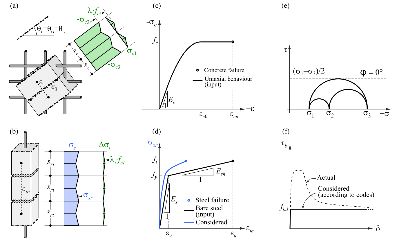
\( \textsf{\textit{\footnotesize{Fig. 1\qquad Basic assumptions of the 3D CSFM: (a) principal stresses in concrete; (b) stresses in the reinforcement direction;}}}\) \( \textsf{\textit{\footnotesize{(c) stress-strain diagram of concrete in terms of maximum stresses; (d) stress-strain diagram of reinforcement}}}\) \( \textsf{\textit{\footnotesize{in terms of stresses at cracks and average strains; (e) Mohr's circles for concrete model in 3D CSFM; (f) bond shear stress-slip}}}\) \( \textsf{\textit{\footnotesize{relationship for anchorage length verifications.}}}\)

Concrete 

The presented material model is a multi-surface plasticity model designed for monotonic loading. It’s important to note that this model does not address unloading, therefore, state variables are not stored, as they would be in classical plasticity models used for cyclic loading.

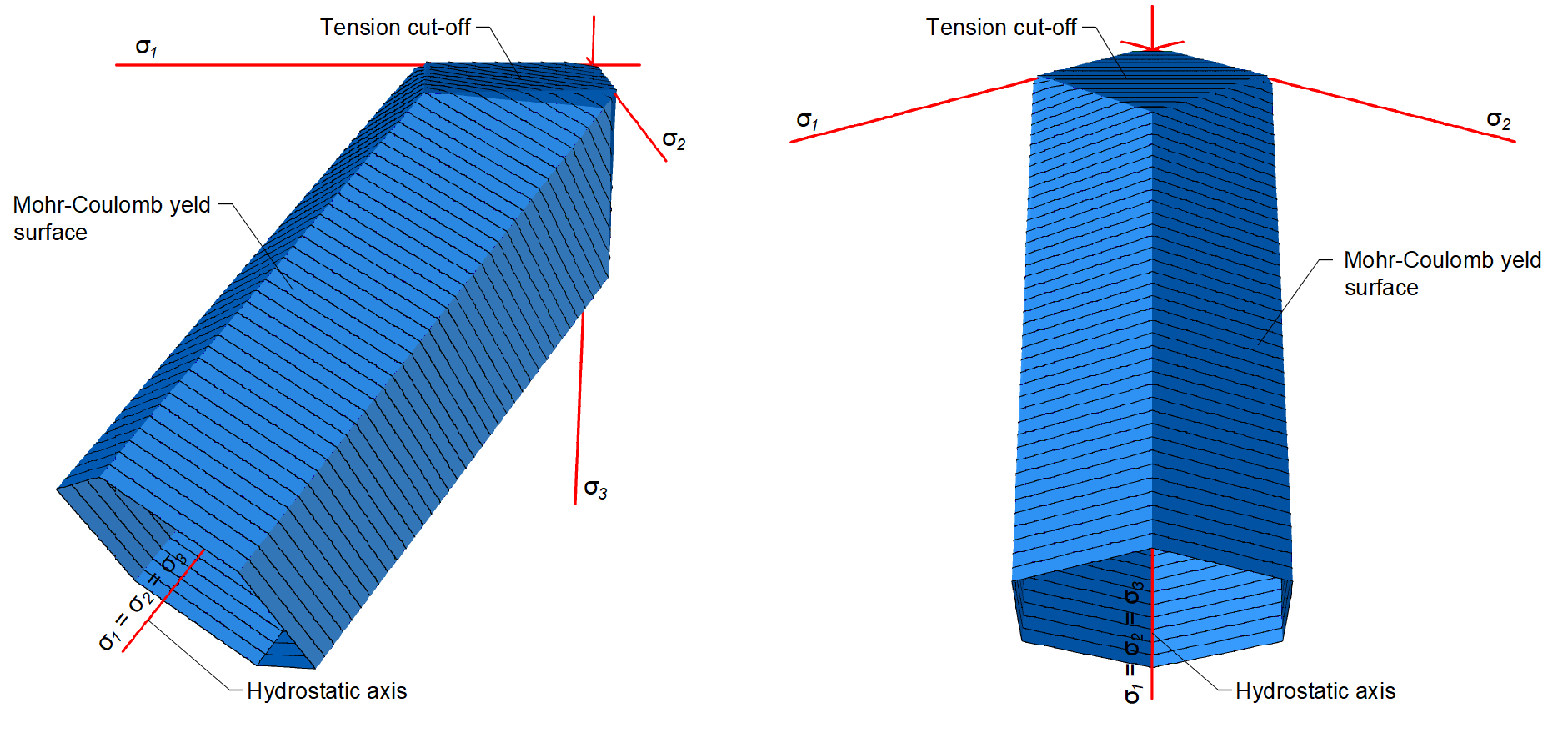
\[ \textsf{\textit{\footnotesize{Fig. 2\qquad Mohr-Coulomb multi-surface plasticity model for friction angle 0 degree}}}\]

As already mentioned, the material model is intended for use in applications that calculate the response of reinforced concrete (not suitable for plain concrete). This is due to the exclusion of concrete in tension. Therefore, the model is not even suitable for structural elements where the design rules for reinforced concrete such as minimum reinforcement ratio, maximum bar spacing, etc., are not fulfilled. It should also be added that, for numerical stability reasons, a very small tensile capacity is defined in the model. The tensile part is restricted by planes corresponding to the Rankine model.

3D CSFM in IDEA StatiCa Detail does not consider an explicit failure criterion in terms of strains for concrete in compression (i.e., it considers an infinitely plastic branch after the peak stress is reached). This simplification does not allow the deformation capacity of structures failing in compression to be verified. However, their ultimate capacity is properly predicted when the increase in the brittleness of concrete as its strength rises is considered by means of the 𝜂_𝑓𝑐 reduction factor defined in fib Model Code 2010 as follows:

\[f_{c,red} = \eta _{fc} \cdot f_{c}\]

\[{\eta _{fc}} = {\left( {\frac{{30}}{{{f_{c}}}}} \right)^{\frac{1}{3}}} \le 1\]

where:

f_c is the concrete cylinder characteristic strength (in MPa for the definition of \( \eta_{fc} \)).

The f_c,red is then compared with the Equivalent Principal Stress σ_c,eq in concrete, which will be defined further, of course, with consideration of all safety factors prescribed by code.

A detailed description of the concrete model can be found at the following link:

• Concrete Material Model for 3D Detail

Reinforcement

The bilinear stress-strain diagram for reinforcement bars, as defined by design codes (Fig. 1d), represents an idealized model. This model necessitates knowledge of the basic properties of the reinforcement during the design phase, specifically the strength and ductility class. Alternatively, users have the option to define a customized stress-strain relationship.

Tension stiffening is considered by modifying the stress-strain relationship of the bare reinforcing bar to capture the average stiffness of the bars embedded in the concrete (ε_m) (Fig 1b).

Anchorage

Bond-slip between reinforcement and concrete is introduced in the finite element model by considering the simplified rigid-perfectly plastic constitutive relationship presented in (Fig. 1f), with f_bd being the design value (factored value) of the ultimate bond stress specified by the design code for the specific bond conditions.

This is a simplified model with the sole purpose of verifying bond prescriptions according to design codes (i.e., anchorage of reinforcement). The reduction of the anchorage length when using hooks, loops, and similar bar shapes can be considered by defining a certain capacity at the end of the reinforcement, as will be described further.

Anchors

In the Beta version of the application, the element of the anchor is defined in the same way as a classical reinforcement. It means that the anchor can transfer only tensile or compressive axial force. The shear can be transferred only by the base plate concrete contact.

Two types of anchors are available:

• Adhesive anchor
• Cast-in-place reinforcement

The Cast-in-place reinforcement behavior is the same as classical reinforcement (Anchorage type, bond, etc.) For Adhesive anchors, it is possible to define the design value Bond strength directly. This value should be read from the technical sheet of the fabricator.

Mohr-Coulomb plasticity theory implementation in 3D CSFM

In the following chapter, we will take a look at how the Mohr-Coulomb theory is implemented in 3D CSFM. We will explain how the confinement effect (triaxial stress) is considered and how the Equivalent Principal Stress σ_c,eq is calculated, which is used to determine the load-bearing capacity from the point of view of concrete.

Introduction to the theory

Mohr–Coulomb theory is a mathematical model describing the response of brittle materials, to shear and normal stress. Most of the classical engineering materials follow this rule in at least a part of their shear failure envelope. Generally, the theory applies to materials for which the compressive strength far exceeds the tensile strength.

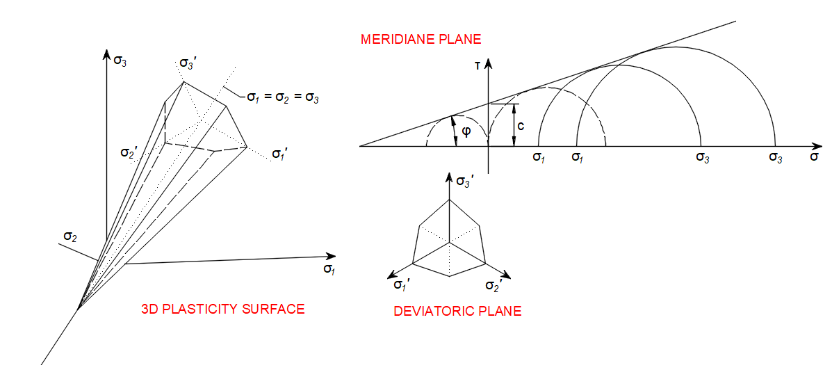
\[ \textsf{\textit{\footnotesize{Fig. 3\qquad Mohr-Coulomb Plasticity Model }}}\]

In structural engineering, it is used to determine failure load as well as the angle of fracture for displacement of fracture surface in concrete and similar materials. Coulomb's friction hypothesis is used to determine the combination of shear and normal stress that will cause a fracture of the material. Mohr's circle is used to determine which principal stresses will produce this combination of shear and normal stress and the angle of the plane in which this will occur. According to the principle of normality, the stress introduced at failure will be perpendicular to the line describing the fracture condition. 

\[ \textsf{\textit{\footnotesize{Fig. 4\qquad Meridian plane and tension cut-off}}}\]

It can be shown that a material failing according to Coulomb's friction hypothesis will show the displacement introduced at failure forming an angle to the line of fracture equal to the angle of friction. This makes the strength of the material determinable by comparing the external mechanical work introduced by the displacement and the external load with the internal mechanical work introduced by the strain and stress at the line of failure. By conservation of energy, the sum of these must be zero and this will make it possible to calculate the failure load of the construction.

Implementation in 3D CSFM

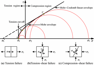
In general, for a given angle of internal friction of the concrete, which is around φ = 30° in Reference [1], [2], [3], [4], the tensile and compressive strengths of the concrete Mohr's circles can be constructed as in Figure 5.

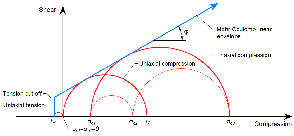
\[ \textsf{\textit{\footnotesize{Fig. 5\qquad Mohr's circles for concrete}}}\]

Where f_c is concrete strength in compression, f_ct is concrete strength in tension, φ is the angle of internal friction, and σ_c1, σ_c3 are the principal stresses of concrete under triaxial compression.

It can be noticed that as the principal stress σ_c3 increases, the maximal possible difference between the values of σ_c3 and σ_c1, which we define as maximal σ_c,eq (see below), also increases.

In 3D CSFM implemented in IDEA StatiCa Detail, the angle of internal friction is considered as φ = 0°, as shown in Figure 6.

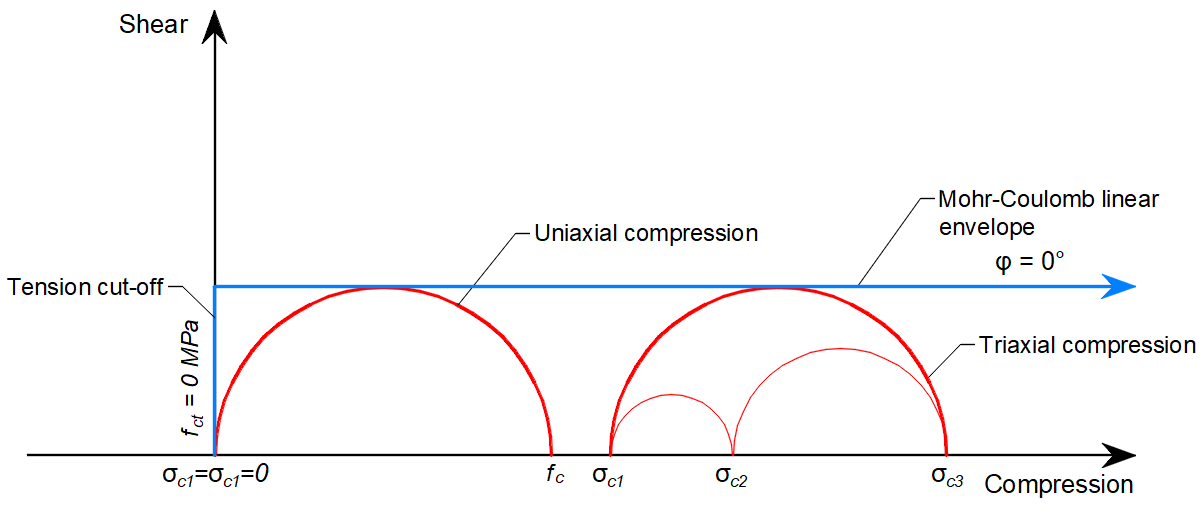
\[ \textsf{\textit{\footnotesize{Fig. 6\qquad Mohr's circles for concrete implemented in IDEA StatiCa Detail}}}\]

The practical consequence of this implementation is that the maximum difference between σ_c3 and σ_c1 is constant as σ_c3 increases. 

Equivalent Principal Stress expresses the equivalent uni-axial stress for a general tri-axial stress state.

\[\sigma_{c,eq} = \sigma_{c3} - \sigma_{c1}\]

The σ_c,eq value can, therefore, be directly compared with uniaxial strength limits according to codes.

Comparing Figure 5, where the real angle of internal friction is used, and Figure 6, which shows the Mohr-Coulomb theory implementation with zero angle of internal friction, it can be seen that the approach chosen for the calculations in Detail is very conservative for the assessment of triaxial stress state.

For a better understanding of the areas affected by tri-axial compression stress, the expression of the increase of the effective material strength due to tri-axial compression has been added to the IDEA StatiCa Detail application as κ factor.

\[\kappa =   \frac{ \sigma_{c3}}{ \sigma_{c,eq}}\]

General mechanics assumptions for 3D CSFM

Equilibrium equations

The theory of small deformations enables the assembly of the equilibrium equation based on the undeformed volume using a first-order approach. 

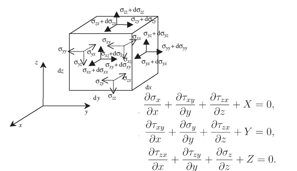
\[ \textsf{\textit{\footnotesize{Fig. 7\qquad Equilibrium equations and graphical representation on infinitesimal element}}}\]

Compatibility equations

A solid body comprises infinitesimal volumes or material points, each of which is interconnected without gaps or overlaps. Mathematical conditions must be adhered to in order to prevent the occurrence of gaps or overlaps when a continuum body undergoes deformation.

Constitutive equations

The constitutive equations governing the behavior of 3D elements play a pivotal role in the analysis of material behavior in structural mechanics. These equations are formulated to accommodate the non-linear isotropic behavior, which is valid for solid block members in IDEA StatiCa Detail. 

When dealing with a 3D wall, it is essential to account for the orthotropic behavior across its thickness, paying particular attention to the tension in the concrete due to the absence of transverse reinforcement. The orthotropy is caused by allowing the tension in concrete in an out-of-plain direction. The material properties such as module elasticity and Poisson ratio remain the same.

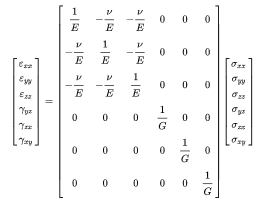
\[ \textsf{\textit{\footnotesize{Fig. 8\qquad Linearly elastic isotropic compliance matrix}}}\]

Analysis model of IDEA StatiCa 3D Detail

An introduction to finite element implementation

3D CSFM considers continuous stress fields in the concrete (3D finite elements), complemented by discrete “rod” elements representing the reinforcement (1D finite elements). Therefore, the reinforcement is not diffusely embedded into the concrete 3D finite elements but explicitly modeled and connected to them. 

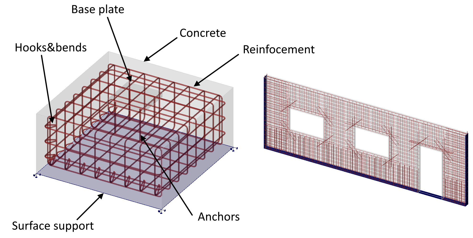
\[ \textsf{\textit{\footnotesize{Fig. 9\qquad Rendering of the calculation model for concrete block and out-of-plane wall}}}\]

Finite element types

The non-linear (inelastic) finite element analysis model is created by several types of finite elements used to model concrete, reinforcement, and the bond between them. Concrete and reinforcement elements are first meshed independently and then interconnected using multi-point constraints (MPC elements). This allows the reinforcement to occupy any position not limited to nodes of tetrahedral mesh. To verify anchorage length, bond, and anchorage end spring elements are inserted between the reinforcement and the MPC elements.

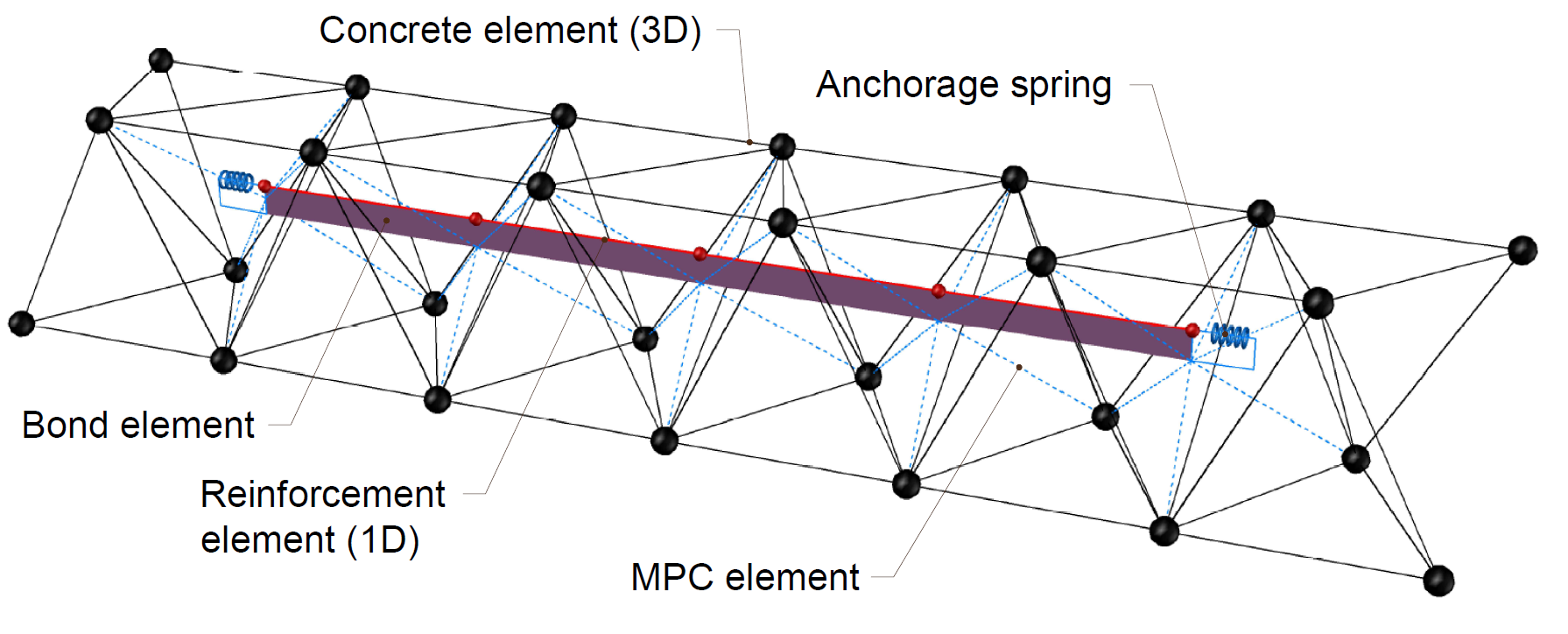
\[ \textsf{\textit{\footnotesize{Fig. 10\qquad Finite element model: reinforcement elements mapped to concrete mesh using MPC and bond elements}}}\]

Concrete

Concrete is analyzed using mixed tetrahedral elements with nodal rotations. The tetrahedral elements allow us to mesh regions of any topology while the implemented formulation guarantees accurate deformation results (without spurious shear stress known as the shear lock effect) even for the coarse mesh which would not be suitable for linear tetrahedral elements formulation. 

Full integration is utilized. It means that each element is equipped with four integration points situated within the volume. Such an integration yields a precise strain and stress field, allowing for sufficient evaluation and presentation of the results across the whole volume. Subsequently, the stop criteria are established based on the value in the integration point.

Reinforcement

Rebars are modeled by two-node 1D “rod” elements (CROD), which only have axial stiffness. These elements are connected to special “bond” elements that were developed in order to model the slip behavior between a reinforcing bar and the surrounding concrete. These bond elements are subsequently connected by MPC (multi-point constraint) elements to the mesh representing the concrete. This approach allows the independent meshing of reinforcement and concrete, while their interconnection is ensured later.

Bond elements

The anchorage length is verified by implementing the bond shear stresses between concrete elements (3D) and reinforcing bar elements (1D) in the finite element model. For this purpose, the “bond” finite element type was developed.

The bond element is defined as a shell finite element connected to elements representing reinforcement by the first layer and by the second layer to concrete mesh via multi-point constraints (MPC elements). It should be noted that the bond element is always displayed in this article with a non-zero height, which is, however, defined as infinitesimal in the model.

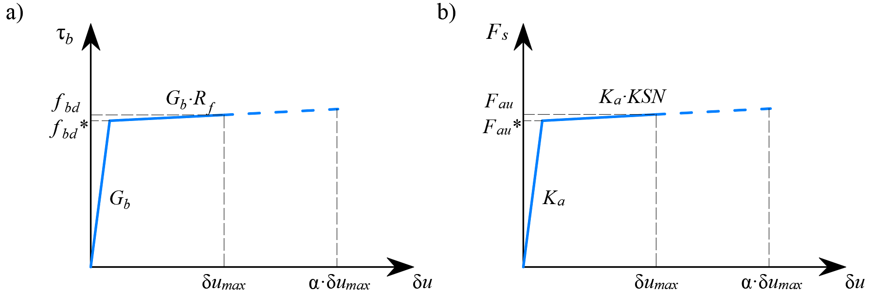
The behavior of this element is described by the bond stress, τ_b, as a bilinear function of the slip between the upper and lower nodes, δu, see (Fig. 11).

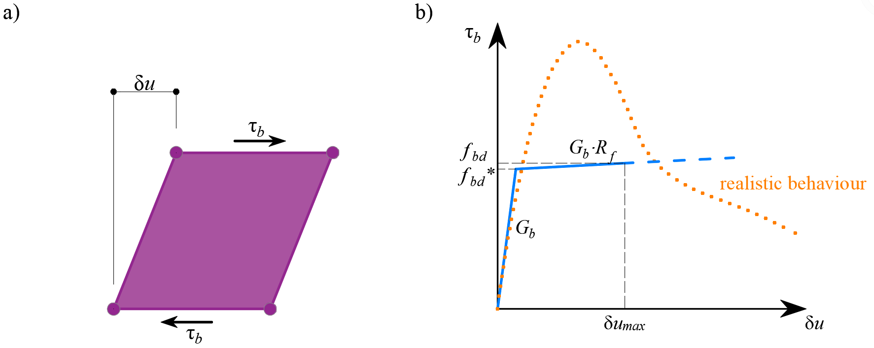
\[ \textsf{\textit{\footnotesize{Fig. 11\qquad (a) Conceptual illustration of the deformation of a bond element; (b) shear-deformation function}}}\]

The elastic stiffness modulus of the bond-slip relationship, Gb, is defined as follows:

\[G_b = k_g \cdot \frac{E_c}{Ø}\]

k_g            coefficient depending on the reinforcing bar surface (by default kg = 0.2)

E_c            modulus of elasticity of concrete (taken as Ecm in case of EN)

Ø             the diameter of the reinforcing bar

The design values (factored values) of ultimate bond shear stress, f_bd, provided in the respective selected design codes EN 1992-1-1 or ACI 318-19 are used to verify the anchorage length. The hardening of the plastic branch is calculated by default as Gb/105.

Anchorage spring

The provision of anchorage ends to the reinforcing bars (i.e., bends, hooks, loops…), which fulfills the prescriptions of design codes, allows the reduction of the basic anchorage length of the bars (l_b,net) by a certain factor β (referred to as the ‘anchorage coefficient’ below). The design value of the anchorage length (lb) is then calculated as follows:

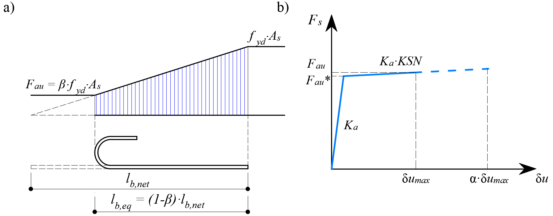
\[ \textsf{\textit{\footnotesize{Fig. 12\qquad Model for the reduction of the anchorage length: a) Anchorage force along the anchorage length of }}}\] \[ \textsf{\textit{\footnotesize{the reinforcement bar, b) slip-anchorage force constitutive law}}}\]

The reduction of the anchorage length is included in the finite element model by means of a spring element at the end of the bar (Fig. 12a), which is defined by the constitutive model shown in (Fig. 12b). The maximum force transmitted by this spring (F_au) is:

\[F_{au} = \beta \cdot A_s \cdot f_{yd}\]

where :

β             the anchorage coefficient based on anchorage type

A_s            the cross-section of the reinforcing bar

f_yd           the design value (factored value) of the yield strength of the reinforcement

Meshing in 3D CSFM

The finite elements are implemented internally, and the analysis model is generated automatically without any need for proficient user interaction. An important part of this process is meshing.

Concrete

All concrete members are meshed together. A recommended element size is automatically computed by the application based on the size and shape of the structure and taking into account the diameter of the largest reinforcing bar. Moreover, the recommended element size guarantees that a minimum of four elements are generated in thin parts of the structure, such as slender columns or thin walls, to ensure reliable results in these areas. Designers can always select a user-defined concrete element size by modifying the multiplier of the default mesh size.

Reinforcement

The reinforcement is divided into elements with approximately the same length as the concrete element size. Once the reinforcement and concrete meshes are generated, they are interconnected with bond elements, as shown in Fig. 9.

The solution method and load-control algorithm for 3D CSFM

A standard full Newton-Raphson (NR) algorithm is used to find the solution to a non-linear FEM problem. 

Generally, the NR algorithm does not often converge when the full load is applied in a single step. A usual approach, which is also used here, is to apply the load sequentially in multiple increments and use the result from the previous load increment to start the Newton solution of the subsequent one. For this purpose, a load control algorithm was implemented on top of the Newton-Raphson. In the case that the NR iterations do not converge, the current load increment is reduced to half its value, and the NR iterations are retried.

A second purpose of the load-control algorithm is to find the critical load, which corresponds to certain “stop criteria” – specifically the maximum strain in concrete, the maximum slip in bond elements, the maximum displacement in anchorage elements, and the maximum strain in reinforcing bars. The critical load is found using the bisection method. In the case where the stop criterion is exceeded anywhere in the model, the results of the last load increment are discarded and a new increment of half the size of the previous one is calculated. This process is repeated until the critical load is found with a certain error tolerance.

For concrete, the stop criterion was set to a 5% strain in compression (i.e., around an order of magnitude larger than the actual failure strain of concrete) and 7% in tension at the integration points of shell elements. In tension, the value was set to allow for the limit strain in reinforcement, which is usually around 5% without accounting for tension stiffening, to be reached first. In compression, the value was chosen from among several alternatives as one that is large enough for the effects of crushing to be visible in the results, but small enough so as not to cause too many problems with numerical stability.

\[ \textsf{\textit{\footnotesize{Fig 13\qquad Constitutive law of bond and anchorage elements used for anchorage length verification: a) Bond shear stress}}}\] \[ \textsf{\textit{\footnotesize{slip response of bond element, b) force-displacement response of an anchorage element}}}\]

For reinforcement, the stop criterion is defined in terms of stresses. Since stresses at the crack are modeled, the criterion in tension corresponds to the reinforcement tensile strength accounting for the safety coefficient. The same value is used for the criterion in compression.

The stop criterion in bond elements and anchorage springs is α·δ_umax, where δ_umax is the maximum slip used in code checks and α = 10.

Presentation of 3D results

The results are presented independently for concrete and for reinforcement elements. The stress and strain values in concrete are calculated at the integration points of volume elements. However, as it is not practical to present the data in such a manner, the results are presented by default in nodes, like the maximum value of compressive stress from adjacent Gauss integration points in connected elements. It should be noted that this representation might locally underestimate the results at compressed edges of members in a case where the finite-element size is similar to the depth of the compression zone.

The results for the reinforcement finite elements are either constant for each element (one value – e.g., for steel stresses) or linear (two values – for bond results). For auxiliary elements, such as elements of bearing plates, only deformations are presented.

Model verification

Limit states

Ultimate limit state

The different verifications required by specific design codes are assessed based on the direct results provided by the model. ULS verifications are carried out for concrete strength, reinforcement strength, and anchorage (bond shear stresses).

To ensure a structural element has an efficient design, it is highly recommended to run a preliminary analysis that takes into account the following steps:

• Choose a selection of the most critical load combinations.
• Calculate only Ultimate Limit State (ULS) load combinations.
• To expedite the calculation time and address any issues, consider using a coarse mesh by increasing the multiplier of the default mesh size in the Setup (Fig. 14). If the model performs well, revert the multiplier back to a factor of 1.

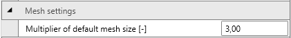
\[ \textsf{\textit{\footnotesize{Fig 14\qquad Mesh multiplier}}}\]

Such a model will calculate very quickly, allowing designers to review the detailing of the structural element efficiently and re-run the analysis until all verification requirements are fulfilled for the most critical load combinations. Once all the verification requirements of this preliminary analysis are fulfilled, it is suggested that the complete ultimate load combinations be included and the use of fine mesh size (the mesh size recommended by the program). Users can change mesh size by the multiplier, which can reach values from 0.5 to 5 (Fig. 14).

The basic results and verifications (stress, strain, and utilization (i.e., the calculated value/limit value from the code)), as well as the direction of principal stresses in the case of concrete elements) are displayed by means of different plots where compression is generally presented in red and tension in blue. Global minimum and maximum values for the entire structure can be highlighted as well as minimum and maximum values for every user-defined part. In a separate tab of the program, advanced results such as tensor values, deformations of the structure, and reinforcement ratios (effective and geometric) used for computing the tension stiffening of reinforcing bars can be shown. Furthermore, loads and reactions for selected combinations or load cases can be presented.

Structural element checks according to Eurocode

Material models in 3D CSFM (EN)

Concrete - ULS

The concrete model implemented in 3D CSFM is based on the uniaxial compression constitutive laws prescribed by EN 1992-1-1 for the design of cross-sections, which only depend on compressive strength. The parabola-rectangle diagram specified in EN 1992-1-1 Cl. 3.1.7 (1) (Fig. 15a) is used by default in 3D CSFM, but designers can also choose a more simplified elastic ideal plastic relationship according to EN 1992-1-1 Cl. 3.1.7 (2) (Fig. 15b). The tensile strength is neglected, as it is in classic reinforced concrete design.

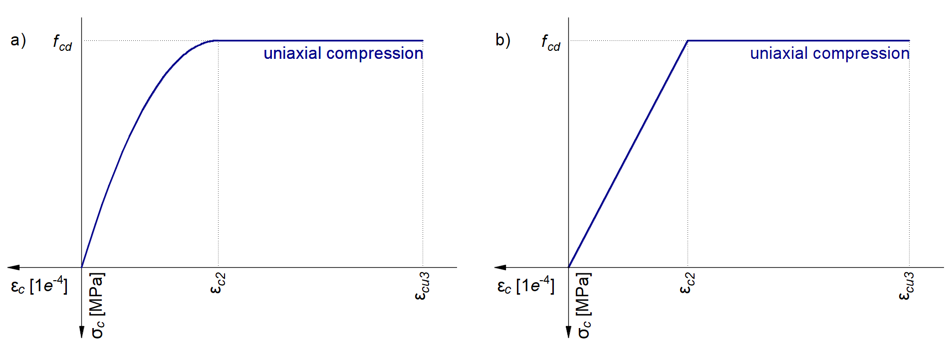
\[ \textsf{\textit{\footnotesize{Fig 15\qquad The stress-strain diagrams of concrete for ULS: a) parabola-rectangle diagram; b) bilinear diagram}}}\]

The implementation of 3D CSFM in IDEA StatiCa Detail does not consider an explicit failure criterion in terms of strains for concrete in compression (i.e., after the peak stress is reached, it considers a plastic branch with ε_cu2 (ε_cu3) in a value of 5% while EN 1992-1-1 assumes ultimate strain less than 0.35%). This simplification does not allow the deformation capacity of structures failing in compression to be verified. However, their ultimate capacity f_cd according to EN 1992-1-1 3.1.3 is properly predicted when the increase in the brittleness of concrete as its strength rises is considered by means of the \(\eta_{fc}\) reduction factor defined in fib Model Code 2010 as follows:

\[f_{cd}={\alpha_{cc}} \cdot \frac{f_{ck,red}}{γ_c} = {\alpha_{cc}} \cdot \frac{\eta _{fc} \cdot f_{ck}}{γ_c}\]

\[{\eta _{fc}} = {\left( {\frac{{30}}{{{f_{ck}}}}} \right)^{\frac{1}{3}}} \le 1\]

where:

α_cc is the coefficient taking account of long-term effects on the compressive strength and of unfavorable effects resulting from the way the load is applied. It is according to EN 1992-1-1 Cl. 3.1.6 (1). The default value is 1.0.

f_ck is the concrete cylinder characteristic strength (in MPa for the definition of \( \eta_{fc} \)).

Reinforcement

By default, the idealized bilinear stress-strain diagram for the bare reinforcing bars defined in EN 1992-1-1, section 3.2.7 (Fig. 16) is considered. The definition of this diagram only requires the basic properties of the reinforcement to be known during the design phase (strength and ductility class). Whenever known, the actual stress-strain relationship of the reinforcement (hot-rolled, cold-worked, quenched, and self-tempered, …) can be considered. The reinforcement stress-strain diagram can be defined by the user, but in this case, it is impossible to assume the tension stiffening effect (it is impossible to calculate crack width). Using the stress-strain diagram with a horizontal top branch does not allow for the verification of structural durability. Therefore, manual verification of standard ductility requirements is necessary.

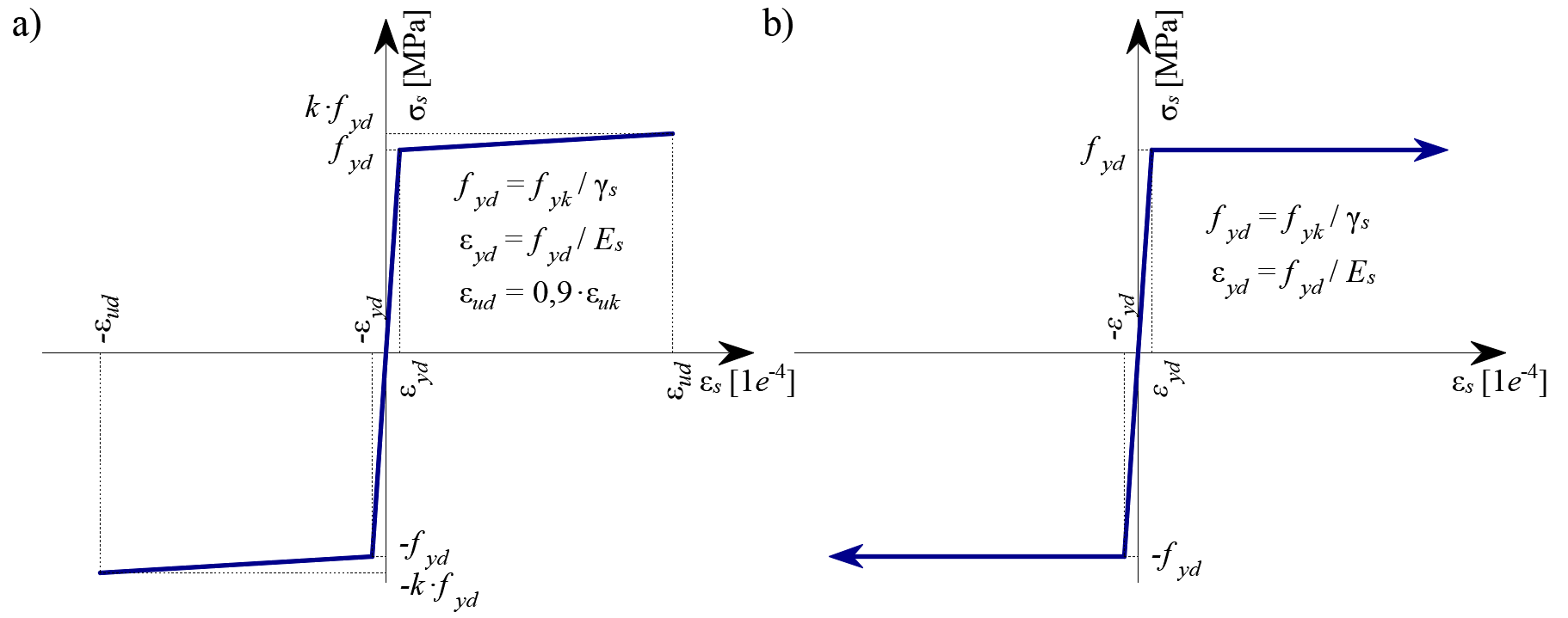
\[ \textsf{\textit{\footnotesize{Fig. 16 \qquad Stress-strain diagram of reinforcement: a) bilinear diagram with an inclined top branch; b) bilinear diagram}}}\] \[ \textsf{\textit{\footnotesize{with a horizontal top branch.}}}\]

Tension stiffening (Fig. 17) is accounted for automatically by modifying the input stress-strain relationship of the bare reinforcing bar in order to capture the average stiffness of the bars embedded in the concrete (ε_m).

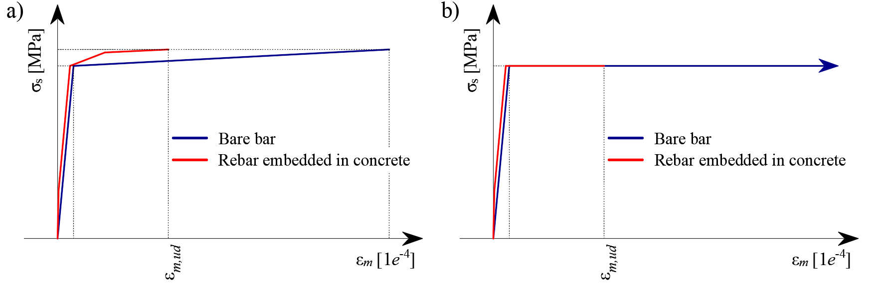
\[ \textsf{\textit{\footnotesize{Fig. 17\qquad Scheme of tension stiffening.}}}\]

Partial safety factors

The Compatible Stress Field Method is compliant with modern design codes. As the calculation models only use standard material properties, the partial safety factor format prescribed in the design codes can be applied without any adaptation. In this way, the input loads are factored, and the characteristic material properties are reduced using the respective safety coefficients prescribed in design codes, exactly as in conventional concrete analysis. Values of material safety factors prescribed in EN 1992-1-1 chap. 2.4.2.4 are set by default, but the user can change safety factors in the Code and calculation settings (Fig. 18).

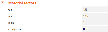
\[ \textsf{\textit{\footnotesize{Fig. 18\qquad The setting of  material safety factors in Idea StatiCa Detail.}}}\]

Load safety factors have to be defined by the user in Combination rules for each non-linear combination of load cases (Fig. 19). For all templates implemented in Idea StatiCa Detail, partial safety factors are already predefined.

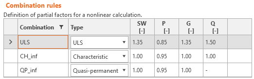
\[ \textsf{\textit{\footnotesize{Fig. 19\qquad The setting of  load partial factors in Idea StatiCa Detail.}}}\]

By using appropriate user-defined combinations of partial safety factors, users can also compute with 3D CSFM using the global resistance factor method (Navrátil, et al. 2017), but this approach is hardly ever used in design practice. Some guidelines recommend using the global resistance factor method for non-linear analysis. However, in simplified non-linear analyses (such as 3D CSFM), which only require those material properties that are used in conventional hand calculations, it is still more desirable to use the partial safety format.

Ultimate limit state checks

The different verifications required by EN 1992-1-1 are assessed based on the direct results provided by the model. ULS verifications are carried out for concrete strength, reinforcement strength, and anchorage (bond shear stresses).

The concrete strength in compression is evaluated as the ratio between the maximum Equivalent principal stress σ_c,eq obtained from FE analysis and the limit value σ_c,lim = f_cd.

Equivalent Principal Stress expresses the equivalent uni-axial stress for a general tri-axial stress state.

\[\sigma_{c,eq} = \sigma_{c3} - \sigma_{c1}\]

The σ_c,eq value can, therefore, be directly compared with uniaxial strength limits according to 1992-1-1 Cl. 3.1.7 (1).

This expression is derived from the implementation of the Mohr-Coulomb plasticity theory, conservatively assuming the angle of internal friction φ = 0°.

The strength of the reinforcement is evaluated in both tension and compression as the ratio between the stress in the reinforcement at the cracks σ_sr and the specified limit value σ_s,lim:

\(σ_{s,lim} = \frac{k \cdot f_{yk}}{γ_s}\qquad\qquad\textsf{\small{for bilinear diagram with inclined top branch}}\)

\(σ_{s,lim} = \frac{f_{yk}}{γ_s}\qquad\qquad\,\,\,\,\textsf{\small{for bilinear diagram with horizontal top branch}}\)

where:

f_yk        is the yield strength of the reinforcement according to EN 1992-1-1 Cl. 3.2.3,

k          is the ratio of tensile strength f_tk to the yield stress,
            \(k = \frac{f_{tk}}{f_{yk}}\)

γ_s             is the partial safety factor for reinforcement.

The bond shear stress is evaluated independently as the ratio between the bond stress τ_b calculated by FE analysis and the ultimate bond strength f_bd, according to EN 1992-1-1 chap. 8.4.2:

\[\frac{τ_{b}}{f_{bd}}\le 1\]

\[f_{bd} = 2.25 \cdot η_1\cdot η_2\cdot f_{ctd}\]

where:

f_ctd      is the design value of concrete tensile strength according to EN 1992-1-1 Cl. 3.1.6 (2). Due to the increasing brittleness of higher-strength concrete, f_ctk,0.05 is limited to the value for C60/75 according to EN 1992-1-1 Cl. 8.4.2 (2)

η₁       is a coefficient related to the quality of the bond condition and the position of the bar during concreting (Fig. 31).

η₁ = 1.0 when ‘good’ conditions are obtained and

η₁ = 0.7 for all other cases and for bars in structural elements built with slip-forms, unless it can be shown that ‘good’ bond conditions exist

η₂        is related to the bar diameter:

            η₂ = 1.0 for Ø ≤ 32 mm

            η₂ = (132 - Ø)/100 for Ø > 32 mm

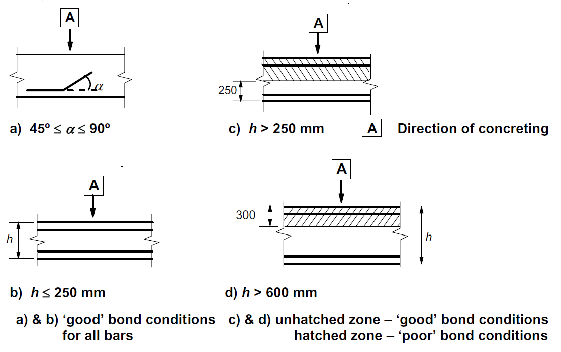
\[ \textsf{\textit{\footnotesize{Fig. 20\qquad EN 1992-1-1 Figure 8.2 - Description of bond conditions.}}}\]

In IDEA StatiCa Detail, the bond conditions are taken into account according to Fig. 20 c) and d). The direction of concreting can be set in the application for each project item as follows:

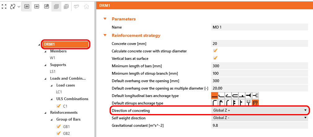
\[ \textsf{\textit{\footnotesize{Fig. 21\qquad Direction of concreating}}}\]

These verifications are carried out with respect to the appropriate limit values for the respective parts of the structure (i.e., in spite of having a single grade both for concrete and reinforcement material, the final stress-strain diagrams will differ in each part of the structure due to tension stiffening and compression softening effects).

Total force F_tot and Limit force F_lim

The total force F_tot is a result of the finite element analysis and can be defined in two ways.

\[F_{tot}=A_{s}\cdot \sigma_{s}\]

where A_s is the area of the reinforcement bar and σ_s is the stress in the bar.

Or as a sum of the anchorage force F_a and the bond force F_bond.

\[F_{tot}=F_{a}+F_{bond}\]

where F_a is the actual force in the anchorage spring and F_bond is the bond force that can be obtained by integrating the bond stress τ_b along the length of reinforcement bar l.

\[F_{bond}=C_{s} \cdot \int_{0}^{l}\tau_{b}\left( x \right)dx\]

C_s is the circumference of the reinforcement bar.

The limit force F_lim is the maximum force in the element of the rebar considering the ultimate strength of the rebar and also anchoring conditions (bond between concrete and reinforcement and anchorage hooks, loops, etc.).

\[F_{lim}=min\left( F_{lim,bond}+F_{au},F_{u} \right)\]

\[F_{u}=k\cdot f_{yd}\cdot A_{s}\]

\[F_{au}=\beta\cdot k\cdot f_{yd}\cdot A_{s}\]

\[F_{lim,bond}=C_{s}\cdot l \cdot f_{bd}\]

where C_s is the circumference of the reinforcement bar, and l is the length from the beginning of the rebar to the point of interest.

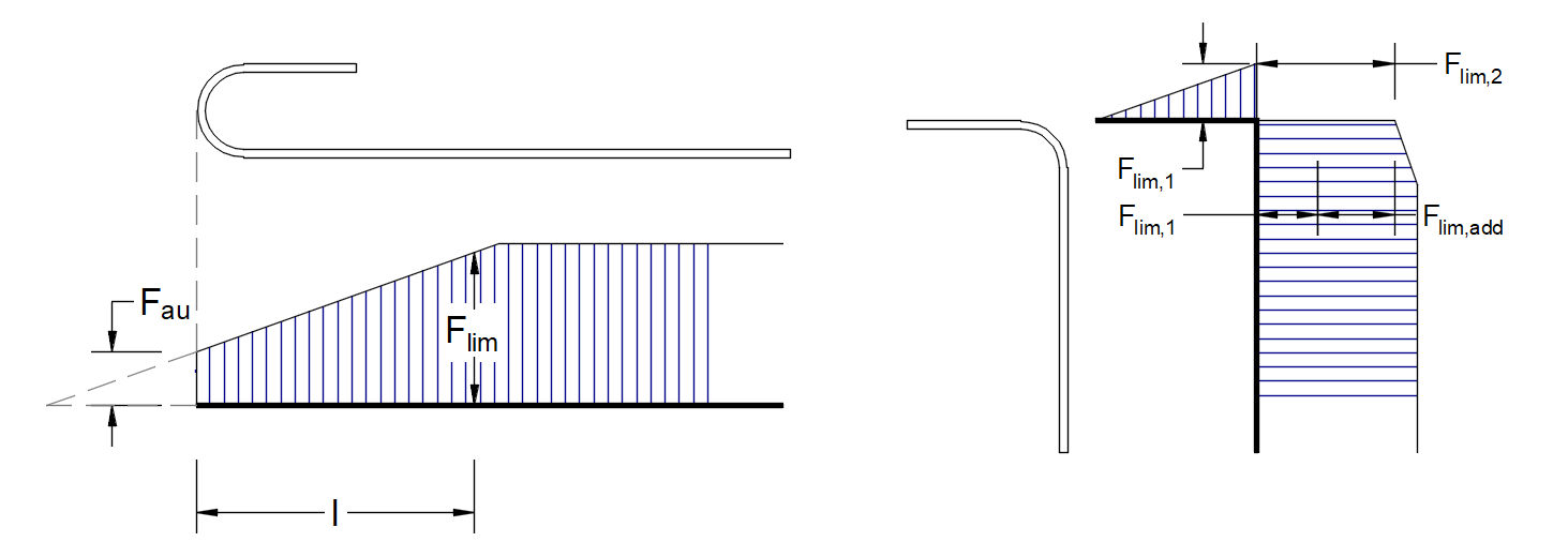
\[ \textsf{\textit{\footnotesize{Fig. 22\qquad Definition of the limit force Flim}}}\]

\[F_{lim,2}=F_{lim,1}+F_{lim,add}\]

where F_lim,add is the additional force calculated from the magnitude of the angle between neighboring elements. F_lim,2 must always be lower than F_u.

The available anchorage types in 3D CSFM include a straight bar (i.e., no anchor end reduction), bend, hook, loop, welded transverse bar, perfect bond, and continuous bar. All these types, along with the respective anchorage coefficients β, are shown in Fig. 23 for longitudinal reinforcement and in Fig. 24 for stirrups. The values of the adopted anchorage coefficients are in accordance with EN 1992-1-1 section 8.4.4 Tab. 8.2. It should be noted that in spite of the different available options, 3D CSFM distinguishes three types of anchorage ends: (i) no reduction in the anchorage length, (ii) a reduction of 30% of the anchorage length in the case of a normalized anchorage, and (iii) perfect bond.

\[ \textsf{\textit{\footnotesize{Fig. 23\qquad  Available anchorage types and respective anchorage coefficients for longitudinal reinforcing bars in the 3D CSFM:}}}\]

\[ \textsf{\textit{\footnotesize{(a) straight bar; (b) bend; (c) hook; (d) loop; (e) welded transverse bar; (f) perfect bond; (g) continuous bar.}}}\]

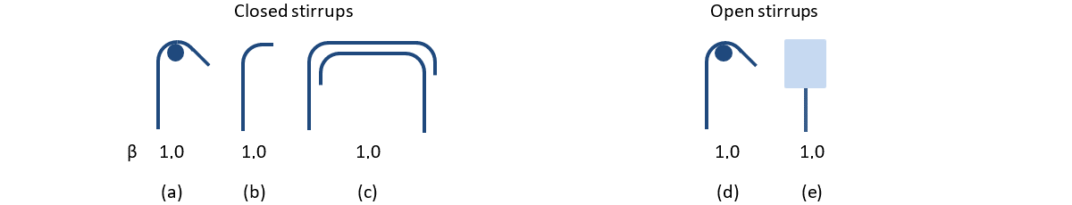
\[ \textsf{\textit{\footnotesize{Fig. 24\qquad  Available anchorage types and respective anchorage coefficients for stirrups.}}}\]

\[ \textsf{\textit{\footnotesize{Closed stirrups: (a) hook; (b) bend; (c) overlap. Open stirrups: (d) hook; (e) continuous bar.}}}\]

In order to comply with EN 1992-1-1, reinforcement must always be modeled with straight ends and the anchorage property must be used (an anchorage spring must be applied). Modeling the anchorage hook by directly modifying the reinforcement geometry is not compliant with EN 1992-1-1.

Verifications and validations

Unit test: Anchoring

Unit test: Simple bending test on cantilevers

Unit test: Shear tests in beams with low amounts of stirrups

References

1. Wu, D.; Wang, Y.; Qiu, Y.; Zhang, J.; Wan, Y.-K. Determination of Mohr–Coulomb Parameters from Nonlinear Strength Criteria for 3D Slopes. Math. Probl. Eng. 2019, 6927654.
2. Lelovic, S.; Vasovic, D.; Stojic, D. Determination of the Mohr-Coulomb Material Parameters for Concrete under Indirect Tensile Test. Tech. Gaz. 2019, 26, 412–419.
3. Galic, M.; Marovic, P.; Nikolic, Ž. Modified Mohr-Coulomb—Rankine material model for concrete. Eng. Comput. 2011, 28, 853–887.
4. Fan, Q.; Gu, S.C.; Wang, B.N.; Huang, R.B. Two Parameter Parabolic Mohr Strength Criterion Applied to Analyze The Results of the Brazilian Test. Appl. Mech. Mater. 2014, 624, 630–634.