Úvod do metody CBFEM
Obecný úvod do konstrukčního návrhu ocelových přípojů
Materiálový model ocelového přípoje
Model plechu a konvergence sítě
Kontakty mezi plechy ocelového přípoje
Analýza svařovaných přípojů
Přípoje se šrouby a předepnutými šrouby
Kotevní šrouby
Konstrukční model betonového bloku
Model analýzy IDEA StatiCa
Model analýzy ocelového styčníku
Rovnováha uzlu v 3D modelu metody konečných prvků
Vnitřní síly v ocelových přípojích
Analýza únosnosti ocelových styčníků
Analýza tuhosti a deformační kapacity ocelových styčníků
Návrh kapacity ocelového přípoje
Návrhová únosnost ocelového přípoje
Analýza boulení ocelového styčníku
Konvergence analýzy složitých modelů ocelových přípojů
Přípoje ocel-dřevo
Tenkostěnné ocelové prvky
Boční torzní ztužení v konstrukčním návrhu
Ocelové styčníky prvků s průřezem dutého profilu
Typ analýzy únavy v konstrukčním návrhu
Návrh na požární odolnost
Dimenzování svarů
Specifikace pro národní normy
Posouzení komponent podle EN (Eurocode)
Posouzení komponent podle AISC (americké normy)
Posouzení komponent podle CISC (kanadské normy)
Posouzení komponent podle AS (australské normy)
Posouzení komponent podle SP (ruské normy)
Posouzení komponent podle IS 800 (indické normy)
Posouzení komponent podle HKG (hongkongský Code of Practice)
Posouzení komponent podle GB (čínské normy)
Úvod do metody CBFEM
Úvod
Prutové prvky jsou inženýry preferovány při navrhování ocelových konstrukcí. Existuje však mnoho míst na konstrukci, kde teorie prutů není platná, např. svařované styčníky, šroubované přípoje, patky, otvory ve stěnách, proměnná výška průřezu a bodová zatížení. Statická analýza v takových místech je obtížná a vyžaduje zvláštní pozornost. Chování je nelineární a nelinearity musí být zohledněny, např. plastifikace materiálu plechů, kontakt mezi čelními deskami nebo patní deskou a betonovým blokem, jednostranné působení šroubů a kotev, svary. Návrhové normy, např. EN1993-1-8, a také odborná literatura nabízejí inženýrské metody řešení. Jejich společným rysem je odvození pro typické konstrukční tvary a jednoduchá zatížení. Velmi často se používá metoda komponent.
Metoda komponent
Metoda komponent (CM) řeší styčník jako soustavu vzájemně propojených prvků – komponent. Odpovídající model je sestaven pro každý typ styčníku tak, aby bylo možné stanovit síly a napětí v každé komponentě – viz následující obrázek.
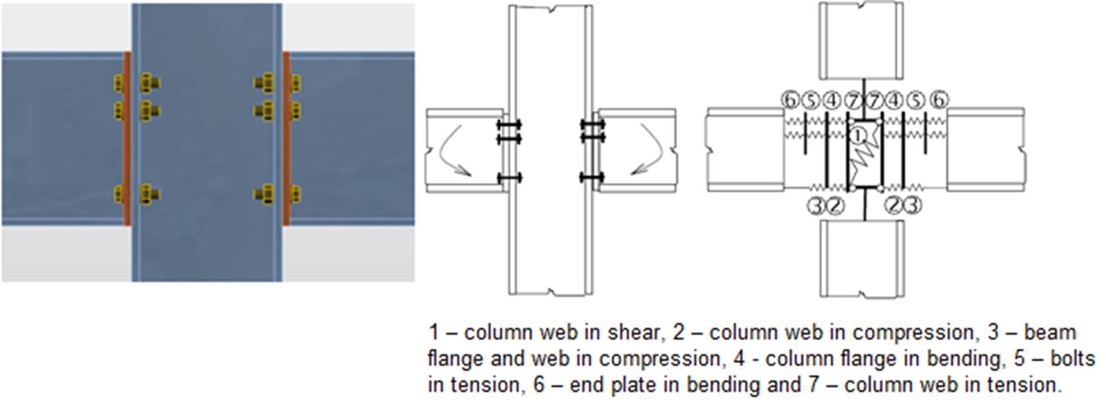
Komponenty styčníku se šroubovanými čelními deskami modelované pružinami
Každá komponenta je posouzena samostatně pomocí příslušných vzorců. Protože pro každý typ styčníku musí být vytvořen odpovídající model, má použití metody omezení při řešení styčníků obecných tvarů a obecných zatížení.
IDEA StatiCa společně s projektovým týmem Katedry ocelových a dřevěných konstrukcí Fakulty stavební v Praze a Ústavu kovových a dřevěných konstrukcí Fakulty stavební Vysokého učení technického v Brně vyvinula metodu pro pokročilý návrh ocelových konstrukčních přípojů.
Component Based Finite Element Model (CBFEM) metoda je:
- Dostatečně obecná, aby byla použitelná pro většinu přípojů, základů a detailů v inženýrské praxi.
- Dostatečně jednoduchá a rychlá v každodenní praxi, aby poskytovala výsledky v čase srovnatelném se současnými metodami a nástroji.
- Dostatečně komplexní, aby poskytovala stavebnímu inženýru jasné informace o chování styčníku, napětí, přetvoření a rezervách jednotlivých komponent a o celkové bezpečnosti a spolehlivosti.
Metoda CBFEM vychází z myšlenky, že většina ověřených a velmi užitečných částí CM by měla být zachována. Slabé místo CM – její obecnost při analýze napětí jednotlivých komponent – bylo nahrazeno modelováním a analýzou pomocí metody konečných prvků (MKP).
MKP je obecná metoda běžně používaná pro statickou analýzu konstrukcí. Použití MKP pro modelování styčníků libovolných tvarů se jeví jako ideální (Virdi, 1999). Je vyžadována elasticko-plastická analýza, protože ocel v konstrukci běžně plastifikuje. Výsledky lineární analýzy jsou pro návrh styčníků prakticky nepoužitelné.
Modely MKP se používají pro výzkumné účely chování styčníků, přičemž obvykle využívají prostorové prvky a naměřené hodnoty vlastností materiálu.
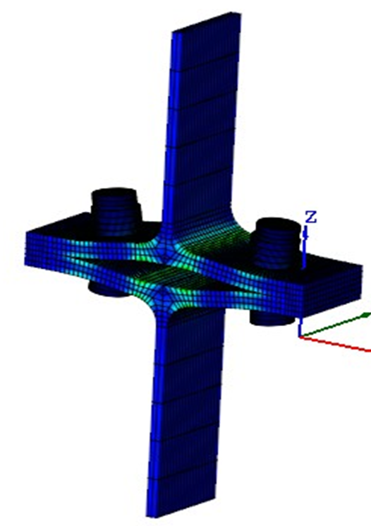
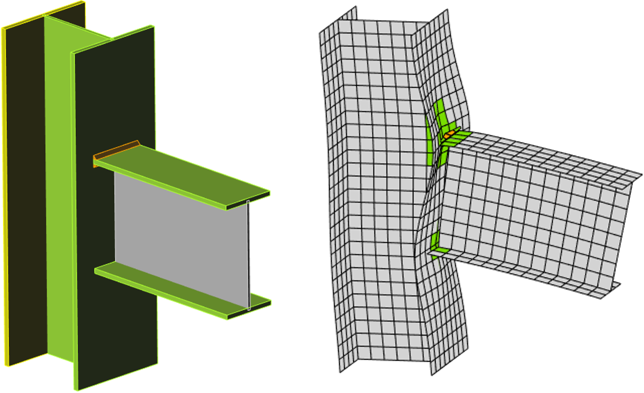
Model MKP styčníku pro výzkumné účely. Používá prostorové 3D prvky jak pro plechy, tak pro šrouby
Stojiny i pásnice připojených prvků jsou v modelu CBFEM modelovány pomocí skořepinových prvků, pro které je k dispozici známé a ověřené řešení.
Spojovací prvky – šrouby a svary – jsou z hlediska analytického modelu nejnáročnější. Modelování těchto prvků v obecných programech MKP je obtížné, protože programy nenabízejí požadované vlastnosti. Proto bylo nutné vyvinout speciální prvky MKP pro modelování chování svarů a šroubů ve styčníku.
Model CBFEM šroubovaného přípoje s čelními deskami
Styčníky prvků jsou při analýze ocelového rámu nebo nosníkové konstrukce modelovány jako bezrozměrné body. V styčnících jsou sestaveny rovnice rovnováhy a po vyřešení celé konstrukce jsou stanoveny vnitřní síly na koncích nosníků. Styčník je ve skutečnosti zatížen těmito silami. Výslednice sil od všech prvků ve styčníku je nulová – celý styčník je v rovnováze.
Skutečný tvar styčníku není ve statickém modelu znám. Inženýr pouze definuje, zda je styčník uvažován jako tuhý nebo kloubový.
Pro správný návrh styčníku je nutné vytvořit věrohodný model styčníku, který respektuje skutečný stav. V metodě CBFEM se používají konce prvků o délce 2–3násobku maximální výšky průřezu. Tyto segmenty jsou modelovány pomocí skořepinových prvků.
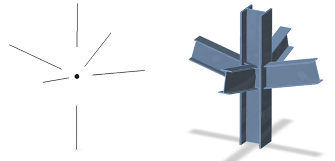
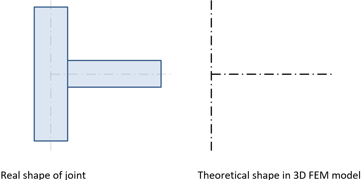
Teoretický (bezrozměrný) styčník a skutečný tvar styčníku bez upravených konců prvků
Pro lepší přesnost modelu CBFEM jsou koncové síly na 1D prvcích přiloženy jako zatížení na koncích segmentů. Šestice sil z teoretického styčníku je přenesena na konec segmentu – hodnoty sil jsou zachovány, ale momenty jsou upraveny o účinky sil na příslušných ramenech.
Konce segmentů ve styčníku nejsou spojeny. Přípoj musí být namodelován. V metodě CBFEM se k modelování přípoje používají tzv. výrobní operace. Výrobními operacemi jsou zejména: řezy, posunutí, otvory, výztuhy, žebra, čelní desky a montážní spoje, úhelníky, styčníkové plechy a další. Jsou také přidány spojovací prvky (svary a šrouby).
IDEA StatiCa Connection může provádět dva typy analýzy:
- Geometricky lineární analýzu s materiálovými a kontaktními nelinearitami pro analýzu napětí a přetvoření,
- Analýzu vlastních čísel pro stanovení možnosti boulení.
V případě přípojů není geometricky nelineární analýza nutná, pokud nejsou plechy velmi štíhlé. Štíhlost plechů lze stanovit analýzou vlastních čísel (boulení). Pro mezní štíhlost, při které je geometricky lineární analýza stále dostačující, viz kapitola 3.9. Geometricky nelineární analýza není v softwaru implementována.
Naučte se efektivně používat IDEA StatiCa s našimi e-learningovými kurzy pro samostudium
Začít se učitNejběžnější materiálové diagramy používané při modelování konstrukční oceli metodou konečných prvků jsou ideálně plastický nebo elastický model se zpevněním a diagram skutečného napětí-přetvoření. Diagram skutečného napětí-přetvoření se vypočítá z materiálových vlastností konstrukční oceli za okolní teploty získaných při tahových zkouškách. Skutečné napětí a přetvoření lze získat takto:
kde σtrue je skutečné napětí, εtrue skutečné přetvoření, σ smluvní napětí a ε smluvní přetvoření.
Plechy v IDEA StatiCa Connection jsou modelovány s elasticko-plastickým materiálem s nominálním sklonem plastického plateau podle EN1993-1-5, čl. C.6, (2), tan-1 (E/1000). Chování materiálu je založeno na von Misesově podmínce plasticity. Předpokládá se elastické chování do dosažení návrhové meze kluzu, fyd.
Kritériem mezního stavu únosnosti pro oblasti, které nejsou náchylné k boulení, je dosažení limitní hodnoty hlavního membránového přetvoření. Doporučuje se hodnota 5 % (např. EN1993-1-5, příl. C, čl. C.8, poznámka 1).
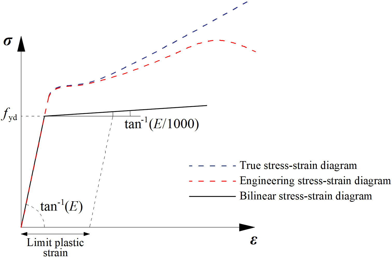
Materiálové diagramy oceli v numerických modelech
Limitní hodnota plastického přetvoření je často předmětem diskuse. Ve skutečnosti má mezní zatížení nízkou citlivost na limitní hodnotu plastického přetvoření při použití ideálně plastického modelu. To je demonstrováno na následujícím příkladu styčníku nosník–sloup. Nosník s otevřeným průřezem IPE 180 je připojen ke sloupu s otevřeným průřezem HEB 300 a zatížen ohybovým momentem. Vliv limitní hodnoty plastického přetvoření na únosnost nosníku je znázorněn na následujícím obrázku. Limitní plastické přetvoření se mění od 2 % do 8 %, přičemž změna momentové únosnosti je menší než 4 %.
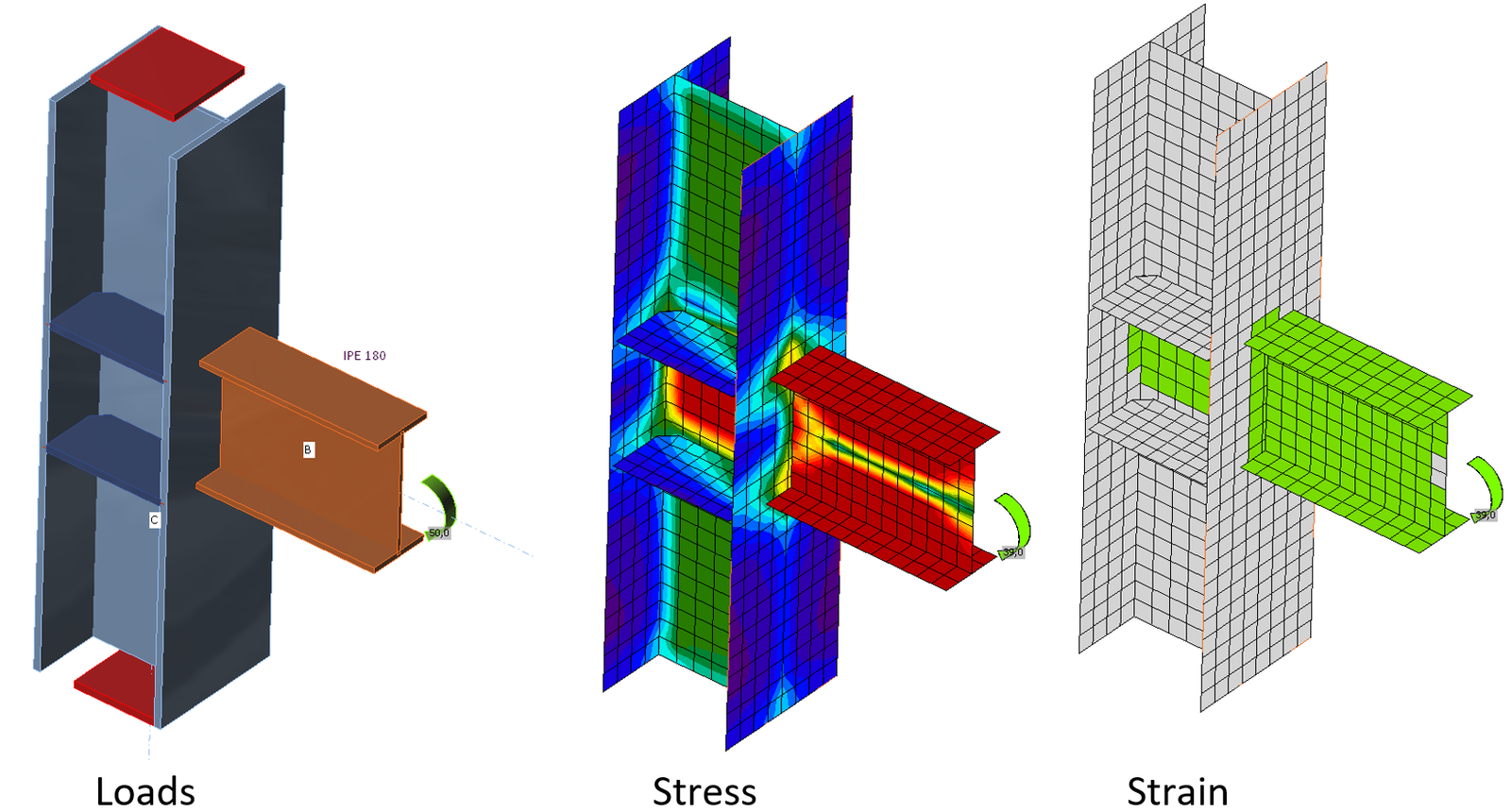
Příklad predikce mezního stavu únosnosti styčníku nosník–sloup
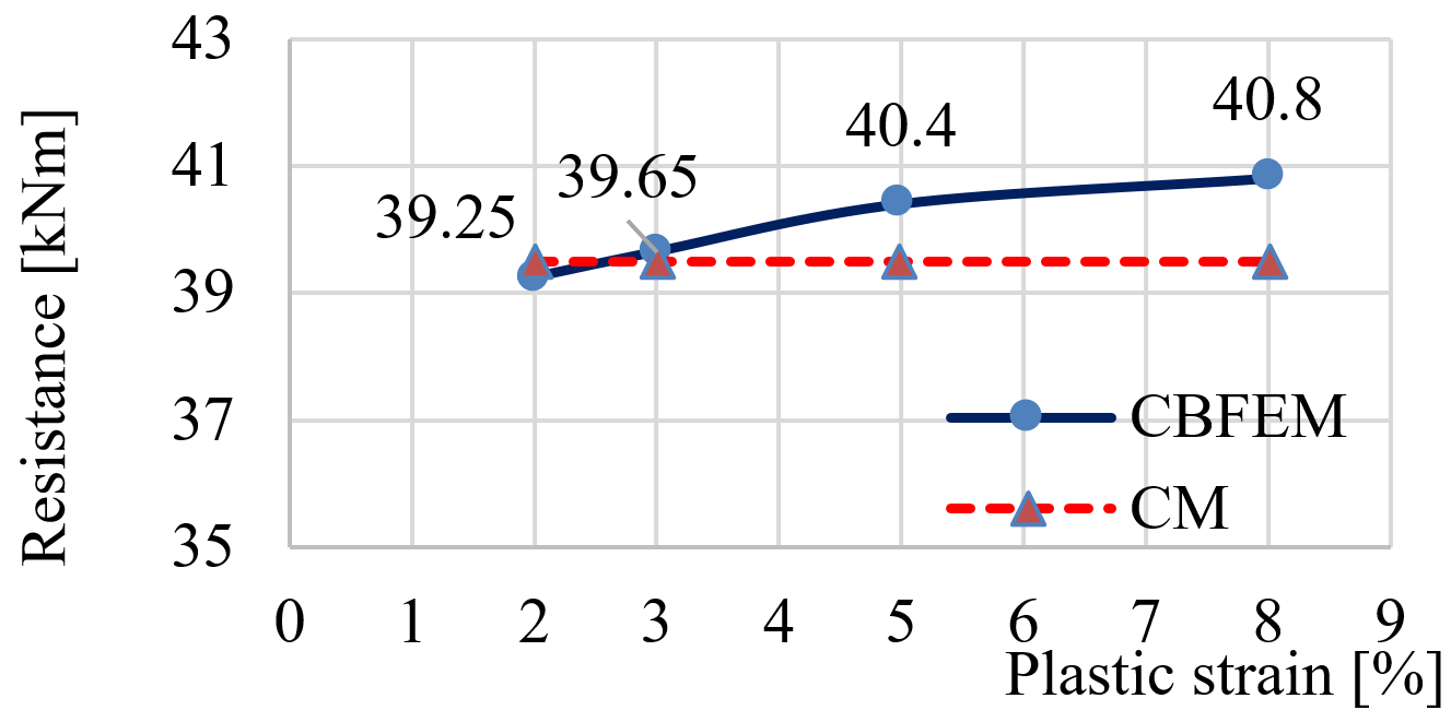
Vliv limitní hodnoty plastického přetvoření na momentovou únosnost
Zvýšení počtu prvků poskytuje přesnější výsledky, ale za cenu vyšší výpočetní náročnosti.
Model plechu
Pro modelování plechů v MKP analýze konstrukčního přípoje se doporučují skořepinové prvky. Jsou použity 4-uzlové čtyřúhelníkové skořepinové prvky s uzly v rozích. V každém uzlu je uvažováno šest stupňů volnosti: 3 posuny (ux, uy, uz) a 3 rotace (φx, φy, φz). Deformace prvku jsou rozděleny na membránovou a ohybovou složku.
Formulace membránového chování vychází z práce Ibrahimbegovice (1990). Jsou uvažovány rotace kolmé na rovinu prvku. Je zajištěna úplná 3D formulace prvku. Smykové deformace mimo rovinu jsou uvažovány ve formulaci ohybového chování prvku na základě Mindlinovy hypotézy. Je použita vlastní stabilizovaná varianta Mindlinova čtyřúhelníkového deskového prvku s konstantní smykovou deformací podél hrany. Prvky jsou inspirovány prvky MITC4; viz Dvorkin (1984). Skořepina je rozdělena do pěti integračních vrstev po tloušťce plechu v každém integračním bodě a plastické chování je analyzováno v každém bodě. Tato metoda se nazývá Gauss–Lobattova integrace. Nelineární elasticko-plastické stadium materiálu je analyzováno v každé vrstvě na základě známých přetvoření. Zobrazena jsou pouze maximální napětí a přetvoření ze všech vrstev.
Konvergence sítě
Pro generování sítě v modelu přípoje existují určitá kritéria. Normové posouzení přípoje by mělo být nezávislé na velikosti prvku. Generování sítě na samostatném plechu je bezproblémové. Pozornost je třeba věnovat složitým geometriím, jako jsou vyztužené panely, T-průřezy a patní desky. Pro složité geometrie by měla být provedena analýza citlivosti s ohledem na diskretizaci sítě.
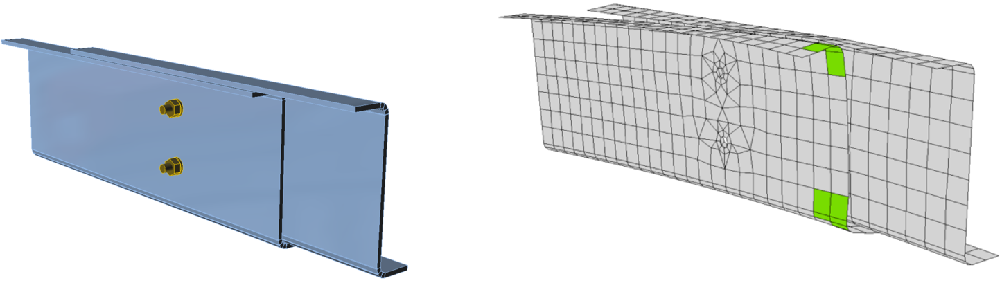
Všechny plechy průřezu nosníku mají společné dělení na prvky. Velikost generovaných konečných prvků je omezena. Minimální velikost prvku je nastavena na 10 mm a maximální velikost prvku na 50 mm (lze nastavit v Nastavení normy). Sítě na přírubách a stojinách jsou na sobě nezávislé. Výchozí počet konečných prvků je nastaven na 8 prvků na výšku průřezu, jak je znázorněno na následujícím obrázku. Uživatel může výchozí hodnoty upravit v Nastavení normy.
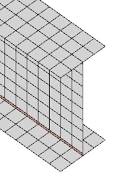
Síť na nosníku s vazbami mezi stojinou a přírubovým plechem
Síť čelních desek je samostatná a nezávislá na ostatních částech přípoje. Výchozí velikost konečného prvku je nastavena na 16 prvků na výšku průřezu, jak je znázorněno na obrázku.
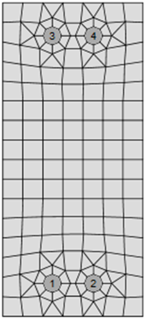
Síť na čelní desce se 7 prvky podél její šířky
Následující příklad styčníku nosník–sloup ukazuje vliv velikosti sítě na momentovou únosnost. Nosník s otevřeným průřezem IPE 220 je připojen ke sloupu s otevřeným průřezem HEA 200 a zatížen ohybovým momentem, jak je znázorněno na následujícím obrázku. Kritickou komponentou je panel stojiny sloupu ve smyku. Počet konečných prvků podél výšky průřezu se mění od 4 do 40 a výsledky jsou porovnány. Přerušované čáry představují rozdíl 5 %, 10 % a 15 %. Doporučuje se rozdělit výšku průřezu na 8 prvků.
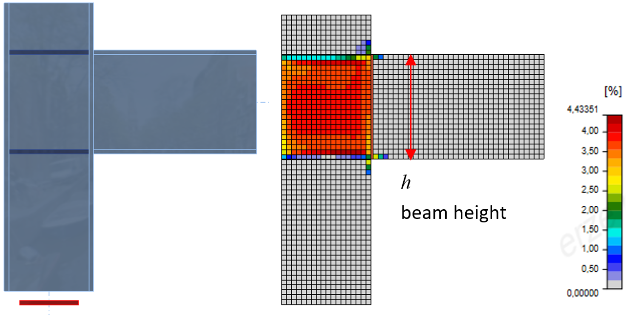
Model styčníku nosník–sloup a plastická přetvoření při mezním stavu únosnosti
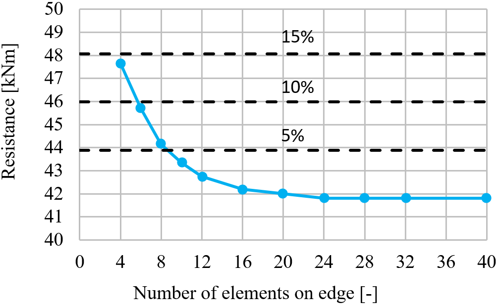
Vliv počtu prvků na momentovou únosnost
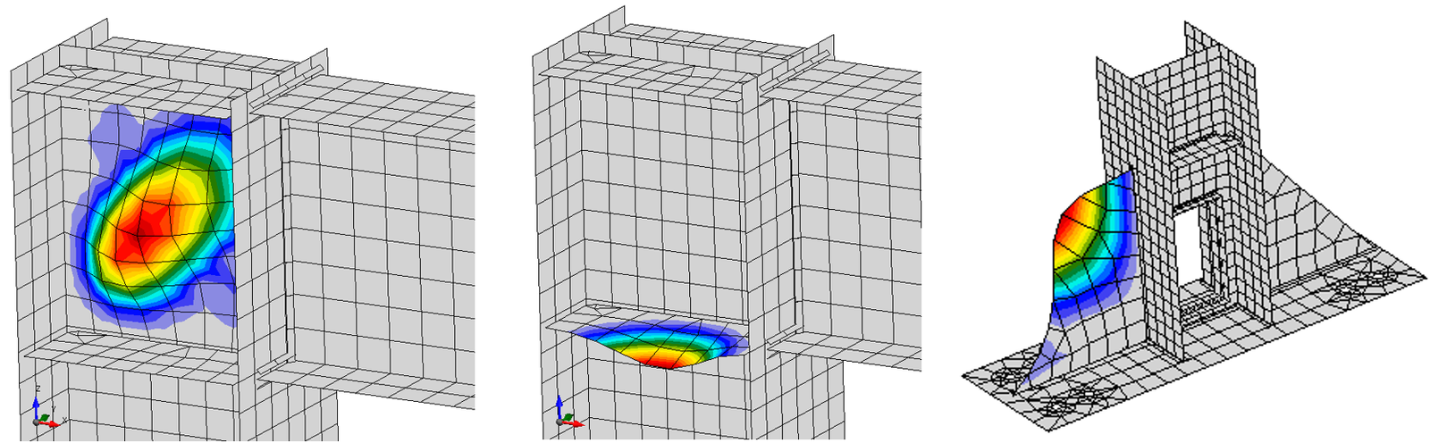
Je prezentována studie citlivosti sítě štíhlé tlačené výztuhy panelu stojiny sloupu. Počet prvků podél šířky výztuhy se mění od 4 do 20. První tvar boulení a vliv počtu prvků na únosnost při boulení a kritické zatížení jsou znázorněny na následujícím obrázku. Je zobrazen rozdíl 5 % a 10 %. Doporučuje se použít 8 prvků podél šířky výztuhy.
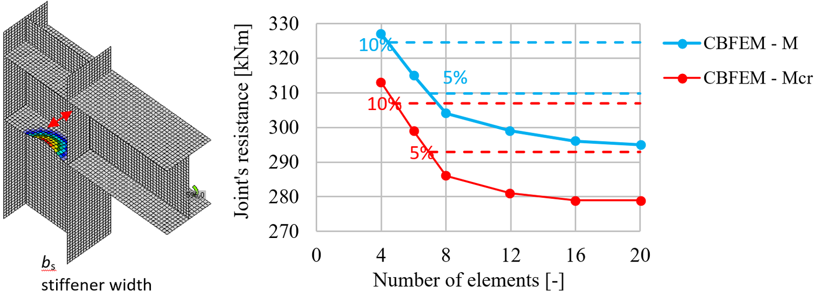
První tvar boulení a vliv počtu prvků podél výztuhy na momentovou únosnost
Je prezentována studie citlivosti sítě T-průřezu v tahu. Polovina šířky příruby je rozdělena na 8 až 40 prvků a minimální velikost prvku je nastavena na 1 mm. Vliv počtu prvků na únosnost T-průřezu je znázorněn na následujícím obrázku. Přerušované čáry představují rozdíl 5 %, 10 % a 15 %. Doporučuje se použít 16 prvků na polovině šířky příruby.
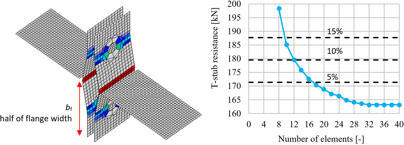
Vliv počtu prvků na únosnost T-průřezu
Pro modelování kontaktu mezi plechy se doporučuje standardní metoda penalizace. Pokud je detekováno proniknutí uzlu do protilehlého kontaktního povrchu, je mezi uzlem a protilehlým plechem přidána penalizační tuhost. Penalizační tuhost je během nelineární iterace řízena heuristickým algoritmem pro dosažení lepší konvergence. Řešič automaticky detekuje bod proniknutí a řeší rozložení kontaktní síly mezi proniknutým uzlem a uzly na protilehlém plechu. To umožňuje vytvoření kontaktu mezi různými sítěmi, jak je znázorněno. Výhodou metody penalizace je automatické sestavení modelu. Kontakt mezi plechy má zásadní vliv na přerozdělení sil v přípoji.
Příklad oddělení plechů v kontaktu mezi stojinou a pásnicemi dvou překrývajících se Z-vaznic
Je možné přidat kontakt mezi
- dvěma povrchy,
- dvěma hranami,
- hranou a povrchem.
Příklad kontaktu hrana-hrana mezi sedlem a čelní deskou
Příklad kontaktu hrana-povrch mezi dolní pásnicí nosníku a pásnicí sloupu
Napětí v kontaktech lze vizualizovat a hodnoty jsou zobrazeny v tabulce posouzení plechů. Kontaktní napětí jsou však pouze informativní a nejsou použita v žádném posouzení. Rovněž není uvažováno napětí skořepinových prvků ve směru tloušťky.
Existuje několik možností, jak zacházet se svary v numerických modelech. Velké deformace činí mechanickou analýzu složitější a je možné použít různé popisy sítě, různé kinetické a kinematické proměnné a konstitutivní modely. Obecně se používají různé typy geometrických 2D a 3D modelů, a tedy konečné prvky s jejich použitelností pro různé úrovně přesnosti. Nejčastěji používaným materiálovým modelem je běžný model plasticity nezávislý na rychlosti deformace, založený na podmínce plasticity von Mises. Jsou popsány dva přístupy používané pro svary. Zbytkové napětí a deformace způsobené svařováním nejsou v návrhovém modelu uvažovány.
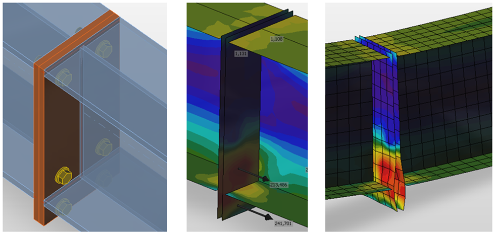
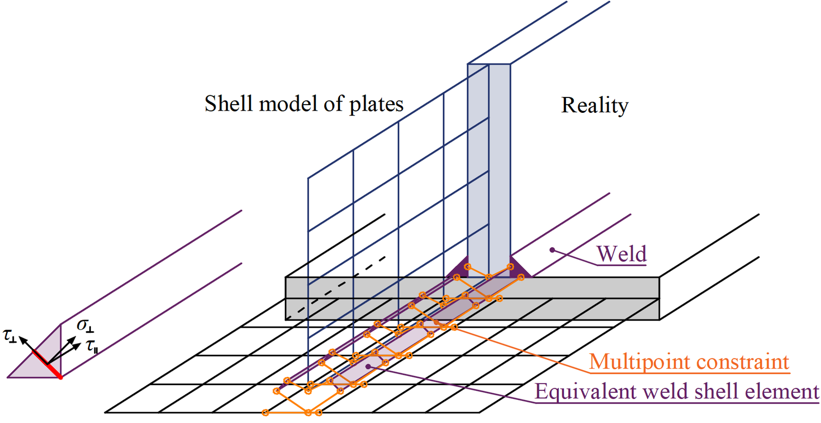
Zatížení je přenášeno prostřednictvím vazeb síla-deformace na základě Lagrangeovy formulace na protilehlý plech. Přípoj je nazýván vazbou více bodů (MPC) a vztahuje uzly konečných prvků jednoho okraje plechu k druhému. Uzly konečných prvků nejsou propojeny přímo. Výhodou tohoto přístupu je schopnost propojit sítě s různými hustotami. Vazba umožňuje modelovat střednicovou plochu spojených plechů s přesazením, které respektuje skutečnou konfiguraci svaru a tloušťku svaru v hrdle. Rozdělení zatížení ve svaru je odvozeno z MPC, takže napětí jsou vypočítána v průřezu hrdla svaru. To je důležité pro rozdělení napětí v plechu pod svarem a pro modelování T-průřezů.
Plastická redistribuce napětí ve svarech
Model pouze s vazbami více bodů nerespektuje tuhost svaru a rozdělení napětí je konzervativní. Špičky napětí, které se objevují na koncích okrajů plechů, v rozích a zaoblení, ovládají únosnost po celé délce svaru. Pro eliminaci tohoto efektu je mezi plechy přidán speciální elastoplastický prvek. Prvek respektuje tloušťku hrdla svaru, polohu a orientaci. Ekvivalentní svarové těleso je vloženo s odpovídajícími rozměry svaru. Je aplikována nelineární materiálová analýza a je stanoveno elastoplastické chování v ekvivalentním svarovém tělese. Stav plasticity je řízen napětími v průřezu hrdla svaru. Špičky napětí jsou redistribuovány podél delší části délky svaru.
Elastoplastický model svarů poskytuje skutečné hodnoty napětí a není třeba napětí průměrovat ani interpolovat. Vypočítané hodnoty v nejvíce namáhaném prvku svaru jsou přímo použity pro posouzení složky svaru. Tímto způsobem není třeba snižovat únosnost vícesměrně orientovaných svarů, svarů k nevyztuženým přírubám ani dlouhých svarů.
Vazba mezi prvkem svaru a uzly sítě
Obecné svary při použití plastické redistribuce lze nastavit jako souvislé, částečné a přerušované. Souvislé svary jsou po celé délce okraje, částečné umožňují uživatelům nastavit přesahy z obou stran okraje a přerušované svary lze navíc nastavit se zadanou délkou a mezerou.
Šrouby
V metodě CBFEM (Component-Based Finite Element Method) je šroub se svým chováním v tahu, smyku a otlačení komponentou popsanou závislými nelineárními pružinami. Sestava šroubu se skládá ze šroubu, podložky a matice a je simulována nelineární pružinou, prvky tuhého tělesa a kontaktními prvky.
Šroub v tahu
Šroub v tahu je popsán pružinou s počáteční osovou tuhostí, návrhovou únosností, inicializací plasticity a deformační kapacitou. Počáteční osová tuhost je analyticky odvozena v normě VDI2230 a v práci Agerskov (1976).
kde:
- – průměr šroubu
- – průměr hlavy šroubu
- – vnitřní průměr podložky
- – vnější průměr podložky
- – součet tlouštěk podložek
- – délka sevření šroubu
- – hrubý průřez šroubu
- – průřez šroubu v tahu
- – Youngův modul pružnosti
Model odpovídá experimentálním datům; viz Gödrich et al. (2014). Pro inicializaci plasticity a deformační kapacitu se předpokládá, že plastická deformace nastává pouze v závitové části dříku šroubu.
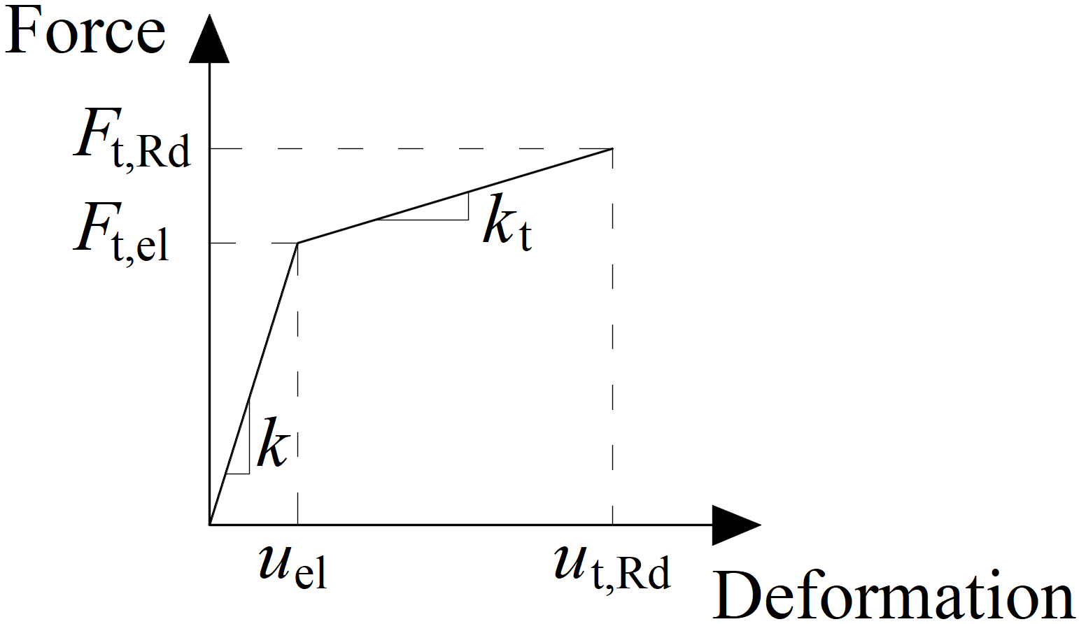
Diagram síla-deformace pro otlačení plechu
Diagram síla-deformace je sestaven pomocí následujících rovnic:
Plastická tuhost:
Síla na mezi pružnosti:
Deformace na mezi pružnosti:
Deformace na mezi plasticity:
kde:
- – návrhová únosnost šroubu v tahu
- – mez kluzu šroubu
- – mez pevnosti šroubu
- – tažnost po přetržení
Šroub ve smyku
Z dříku šroubu na plech v otvoru šroubu se přenáší pouze tlaková síla. Je modelována interpolačními vazbami mezi uzly dříku a uzly na hraně otvoru. Deformační tuhost skořepinového prvku modelujícího plechy rozděluje síly mezi šrouby a simuluje odpovídající otlačení plechu.
Otvory pro šrouby jsou uvažovány jako standardní (výchozí) nebo podlouhlé (lze nastavit v editoru plechu). Šrouby ve standardních otvorech mohou přenášet smykovou sílu ve všech směrech, šrouby v podlouhlých otvorech mají jeden směr vyloučen a mohou se v tomto zvoleném směru volně pohybovat.
Počáteční tuhost a návrhová únosnost šroubu ve smyku jsou definovány následujícími vzorci:
kde:
- – průměr šroubu
- – mez pevnosti šroubu
- – průměr referenčního šroubu M16
- – mez pevnosti připojeného plechu
- – minimální tloušťka připojeného plechu
Pružina reprezentující šroub ve smyku má bilineární chování síla-deformace. Inicializace plasticity se předpokládá při:
Deformační kapacita je uvažována jako:
kde:
- – pružná únosnost šroubu ve smyku
- – únosnost šroubu ve smyku
- – pružná deformace šroubu ve smyku
Interakce tahu a smyku
Interakce osové a smykové síly může být zavedena přímo do výpočetního modelu. Rozdělení sil lépe odpovídá skutečnosti (viz přiložený diagram). Šrouby s vysokou tahovou silou přenášejí menší smykovou sílu a naopak.
Příklad interakce osové a smykové síly (EC)
Předepnuté šrouby
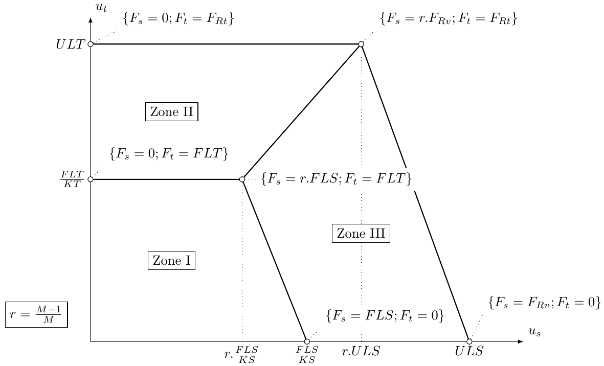
Předepnuté šrouby se používají v případech, kdy je nutné minimalizovat deformace. Model šroubu v tahu je stejný jako u standardních šroubů. Smyková síla se nepřenáší otlačením, ale třením mezi sevřenými plechy.
Návrhová únosnost předepnutého šroubu v prokluzu je ovlivněna působící tahovou silou.
IDEA StatiCa Connection posuzuje mezní stav před prokluzem předepnutých šroubů. Pokud dojde k prokluzu, šrouby nevyhoví posouzení. V takovém případě je třeba posoudit mezní stav po prokluzu jako standardní posouzení šroubů na otlačení, kde jsou otvory pro šrouby namáhány otlačením a šrouby smykem.
Uživatel může rozhodnout, který mezní stav bude posuzován. Buď se jedná o únosnost proti hlavnímu prokluzu, nebo o stav po prokluzu při smyku šroubů. Obě posouzení na jednom šroubu nejsou v jednom řešení kombinována. Předpokládá se, že šroub má po hlavním prokluzu standardní chování a může být posouzen standardním postupem na otlačení.
Momentové zatížení přípoje má malý vliv na smykovou únosnost. Přesto je posouzení tření na každém šroubu řešeno samostatně. Toto posouzení je implementováno v komponentě šroubu metodou konečných prvků. Obecně není k dispozici informace o tom, zda vnější tahové zatížení každého šroubu pochází z ohybového momentu nebo z tahového zatížení přípoje.
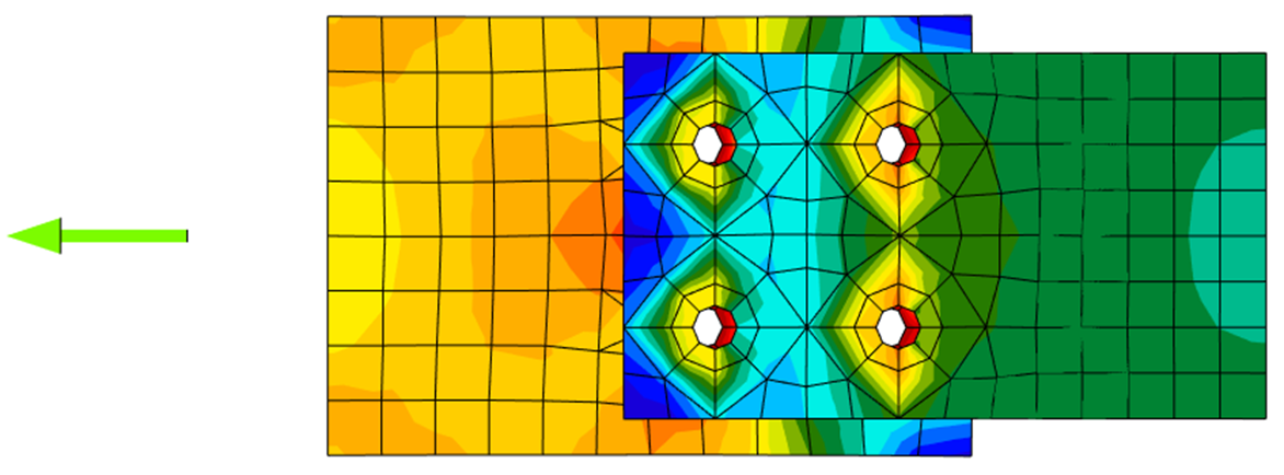
Rozdělení napětí ve standardním smykovém šroubovém přípoji
Rozdělení napětí ve smykovém šroubovém přípoji odolném proti prokluzu
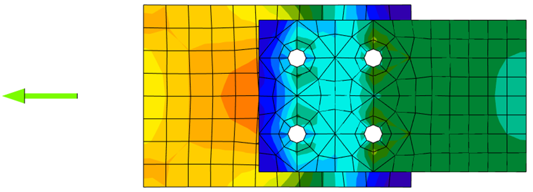
Kotevní šroub je modelován podobnými postupy jako konstrukční šrouby. Šroub je na jedné straně betonového bloku pevně uchycen. Jeho délka, Lb, používaná pro výpočet tuhosti šroubu, je rovna součtu poloviny tloušťky matice, tloušťky podložky, tw, tloušťky patní desky, tbp, tloušťky podlití nebo mezery, tg, a volné délky zabetonované v betonu, která se předpokládá jako 8d, kde d je průměr šroubu. Faktor 8 je editovatelný v nastavení normy. Tato hodnota je v souladu s komponentovou metodou (EN1993-1-8); volná délka zabetonovaná v betonu může být upravena v nastavení normy. Tuhost v tahu se vypočítá jako k = E As / Lb. Diagram zatížení-deformace kotevního šroubu je znázorněn na následujícím obrázku. Hodnoty podle ISO 898:2009 jsou shrnuty v tabulce a ve vzorcích níže.
Diagram zatížení–deformace kotevního šroubu
kde:
- A – tažnost
- E – Youngův modul pružnosti
- Ft,Rd – návrhová únosnost kotvy v tahu
- Rm – mez pevnosti (v tahu)
- Re – mez kluzu
Tuhost kotevního šroubu ve smyku je uvažována jako tuhost konstrukčního šroubu ve smyku.
Kotevní šrouby s volnou délkou (stand-off)
Kotvy s volnou délkou lze posoudit jako fázi výstavby před podlitím patky sloupu nebo jako trvalý stav. Kotva s volnou délkou je navržena jako prutový prvek zatížený smykovou silou, ohybovým momentem a tlakovou nebo tahovou silou. Kotva je na obou stranách pevně uchycena; jedna strana je 0,5×d pod úrovní betonu, druhá strana je uprostřed tloušťky plechu. Vzpěrná délka je konzervativně uvažována jako dvojnásobek délky prutového prvku. Používá se plastický průřezový modul. Síly v kotvě s volnou délkou jsou stanoveny pomocí metody konečných prvků. Ohybový moment závisí na poměru tuhostí kotev a patní desky.
Kotvy s volnou délkou – stanovení ramene síly a vzpěrných délek; tuhé kotvy jsou konzervativním předpokladem
Návrhový model
V CBFEM je vhodné zjednodušit betonový blok jako 2D kontaktní prvky. Spojení mezi betonem a patní deskou přenáší pouze tlak. Tlak je přenášen prostřednictvím modelu podloží Winkler-Pasternak, který reprezentuje deformace betonového bloku. Tahová síla mezi patní deskou a betonovým blokem je přenášena kotevními šrouby. Smyková síla je přenášena třením mezi patní deskou a betonovým blokem, smykovou zarážkou a ohybem kotevních šroubů a třením. Únosnost šroubů ve smyku je posuzována analyticky. Tření a smyková zarážka jsou modelovány jako plná jednobodová podpora v rovině kontaktu patní desky s betonem.
Deformační tuhost
Tuhost betonového bloku lze pro návrh patek sloupů odhadnout jako elastickou polokouli. Model podloží Winkler-Pasternak se běžně používá pro zjednodušený výpočet základů. Tuhost podloží je stanovena pomocí modulu pružnosti betonu a efektivní výšky podloží jako:
kde:
- k – tuhost betonového podloží v tlaku
- Ec – modul pružnosti betonu
- υ – Poissonův součinitel betonového bloku
- Aeff – efektivní plocha v tlaku
- Aref = 1 m2 – referenční plocha
- d – šířka patní desky
- h – výška betonového bloku
- a1 = 1,65; a2 = 0,5; a3 = 0,3; a4 = 1,0 – součinitele
Ve vzorci musí být použity jednotky SI, výsledná jednotka je N/m3.
Přenos smykového zatížení v patní desce
Smykové zatížení v patní desce lze přenést třemi způsoby:
- Třením
- Smykovou zarážkou
- Kotvami
Uživatelé mohou zvolit způsob přenosu úpravou operace patní desky. Kombinace způsobů přenosu není v softwaru povolena, avšak EN 1993-1-8 – čl. 6.2.2 a Fib 58 – kapitola 4.2 umožňují kombinaci přenosu smyku kotvami a třením za určitých podmínek. Obecně je konzervativní zanedbat tření při návrhu kotvení, i když to může v některých případech vést k podhodnocení trhlin v betonu na úrovni MSP. Zpravidla by měla být třecí únosnost zanedbána, pokud:
- tloušťka zálivkové vrstvy přesahuje polovinu průměru kotvy,
- kapacita kotvení je řízena podmínkou blízkosti hrany,
- kotvení je navrženo k přenosu seismického zatížení.
Kombinace se smykovou zarážkou by nikdy neměla být povolena z důvodu deformační kompatibility.
Přenos smykového zatížení třením
Smyková únosnost se rovná součinu dílčího součinitele únosnosti, součinitele tření (upravitelného v nastavení normy) a tlakového zatížení. Tlakové zatížení zahrnuje všechny síly – například v případě patky sloupu zatížené tlakovou silou a ohybovým momentem může být tlakové zatížení použité pro třecí smykovou únosnost vyšší než působící tlaková síla.
Přenos smykového zatížení smykovou zarážkou
Smyková zarážka je simulována jako pahýl zabetonovaný v betonu pod patní deskou. Předpokládá se, že smykové zatížení je přenášeno rovnoměrným rozložením zatížení působícím na celou část smykové zarážky zabetonované v betonovém bloku, tj. všechny uzly smykové zarážky pod povrchem betonu jsou rovnoměrně zatíženy. Část smykové zarážky nad povrchem betonu v zálivce se nepředpokládá jako přenášející smykové zatížení.
Je třeba si uvědomit, že rameno mezi působícím smykovým zatížením (v patní desce) a smykovou únosností (v polovině výšky smykové zarážky zabetonované v betonu) způsobuje ohybový moment, který musí být přenesen tlakovou silou v betonu a tahovými silami v kotvách.
Smyková zarážka se skládá ze skořepinových konečných prvků a je posuzována jako běžný plech. Rovněž svary smykové zarážky k patní desce jsou posuzovány standardními postupy v IDEA StatiCa Connection. Ruční výpočet obvykle předpokládá pro smykovou zarážku teorii nosníku, i když není přesná, protože poměr délky k šířce je u smykové zarážky velmi malý. Proto může být mezi IDEA StatiCa Connection a ručním výpočtem významný rozdíl.
Přenos smykového zatížení kotvami
Smyková únosnost je stanovena smykovou únosností kotev. Ocelová únosnost kotev má elastoplastickou křivku zatížení-deformace, avšak způsoby porušení betonu jsou uvažovány jako dokonale křehké.
Model analýzy IDEA StatiCa
Metoda CBFEM (Component Based Finite Element Model) umožňuje rychlou analýzu styčníků různých tvarů a konfigurací. Model se skládá z prvků, na které je aplikováno zatížení, a výrobních operací (včetně ztužujících prvků), které slouží ke vzájemnému propojení prvků. Prvky nesmí být zaměňovány s výrobními operacemi, protože jejich řezné hrany jsou připojeny přes tuhé vazby k uzlu přípoje, takže se při použití místo výrobních operací (ztužujících prvků) správně nedeformují.
Analyzovaný model MKP je generován automaticky. Návrhář nevytváří model MKP, ale vytváří styčník pomocí výrobních operací – viz obrázek.
Výrobní operace/položky, které lze použít ke konstrukci styčníku
Každá výrobní operace přidává do přípoje nové položky – řezy, plechy, šrouby, svary.
Nosné prvky a podpory
Jeden prvek styčníku je vždy nastaven jako „nosný". Všechny ostatní prvky jsou „připojené". Nosný prvek může zvolit návrhář. Nosný prvek může být ve styčníku „průběžný" nebo „ukončený". „Ukončené" prvky jsou podepřeny na jednom konci a „průběžné" prvky jsou podepřeny na obou koncích.
Připojené prvky mohou být několika typů podle zatížení, které je prvek schopen přenést:
- Typ N-Vy-Vz-Mx-My-Mz – prvek je schopen přenést všech 6 složek vnitřních sil
- Typ N-Vy-Mz – prvek je schopen přenést pouze zatížení v rovině XY – vnitřní síly N, Vy, Mz
- Typ N-Vz-My – prvek je schopen přenést pouze zatížení v rovině XZ – vnitřní síly N, Vz, My
- Typ N-Vy-Vz – prvek je schopen přenést pouze normálovou sílu N a posouvající síly Vy a Vz
Přípoj plech na plech přenáší všechny složky vnitřních sil
Přípoj žiletkou může přenášet pouze zatížení v rovině XZ – vnitřní síly N, Vz, My
Styčníkový přípoj – přípoj prvku příhradové konstrukce může přenášet pouze osovou sílu N a posouvající síly Vy a Vz
Každý styčník je během analýzy rámové konstrukce ve stavu rovnováhy. Pokud jsou na podrobný model CBFEM aplikovány koncové síly jednotlivých prvků, je stav rovnováhy rovněž splněn. Nebylo by tedy nutné definovat podpory v analytickém modelu. Z praktických důvodů je však na prvním konci nosného prvku definována podpora bránící všem posunům. Tato podpora neovlivňuje ani stav napětí, ani vnitřní síly ve styčníku, pouze prezentaci deformací.
Na koncích připojených prvků jsou definovány odpovídající typy podpor respektující typ jednotlivých prvků, aby se zabránilo vzniku nestabilních mechanismů.
Výchozí délka každého prvku je dvojnásobek jeho výšky. Délka prvku by měla být po poslední výrobní operaci (svar, otvor, výztuha atd.) nejméně 1× výška prvku, a to z důvodu správných deformací za tuhými vazbami spojujícími řezný konec prvku s uzlem přípoje.
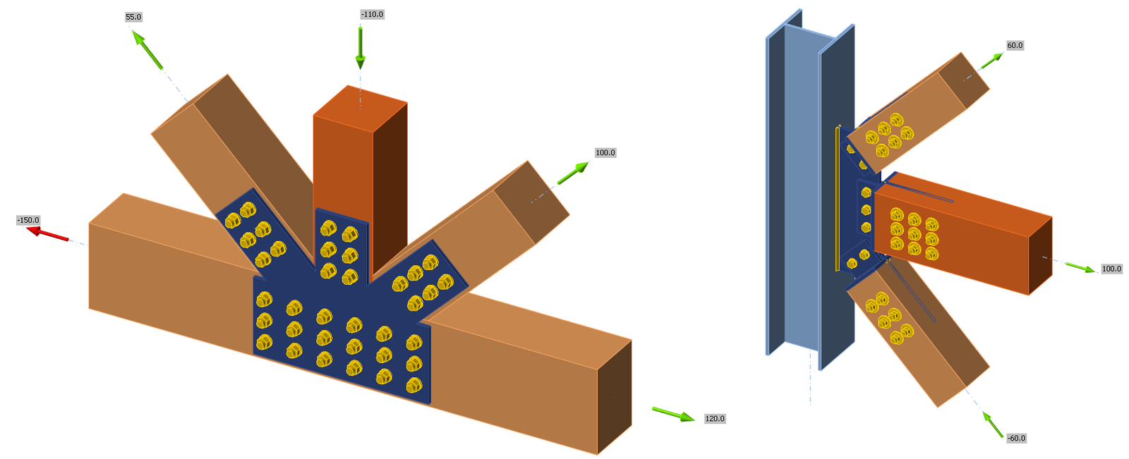
Zatížení v každém uzlu konstrukčního modelu musí být v rovnováze. Jakékoli nevyvážené síly jsou přenášeny podporami. Doporučuje se používat kombinaci zatížení místo obálky vnitřních sil.
Každý uzel 3D modelu metody konečných prvků musí být v rovnováze. Požadavek na rovnováhu je správný, nicméně není nutný pro návrh jednoduchých styčníků. Jeden prvek styčníku je vždy „nosný" a ostatní jsou připojeny. Pokud je kontrolováno pouze připojení připojených prvků, není nutné dodržovat rovnováhu. K dispozici jsou tedy dva režimy zadávání zatížení:
- Zjednodušený – v tomto režimu je nosný prvek podepřen (průběžný prvek na obou stranách) a zatížení není na prvku definováno
- Pokročilý (přesný s kontrolou rovnováhy) – nosný prvek je podepřen na jednom konci, zatížení je aplikováno na všechny prvky a musí být nalezena rovnováha
Režim lze přepínat ve skupině pásu karet Zatížení v rovnováze.

Rozdíl mezi režimy je ukázán na následujícím příkladu T-přípoje. Nosník je zatížen koncovým ohybovým momentem 41 kNm. Ve sloupu působí také tlaková normálová síla 100 kN. V případě zjednodušeného režimu není normálová síla zohledněna, protože sloup je podepřen na obou koncích. Program zobrazuje pouze účinek ohybového momentu nosníku. Účinky normálové síly jsou analyzovány pouze v plném režimu a jsou zobrazeny ve výsledcích.
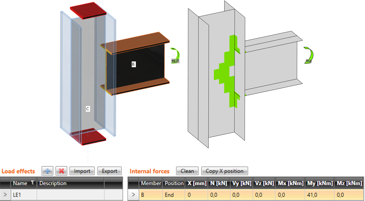
Zjednodušené zadání: normálová síla ve sloupu NENÍ zohledněna
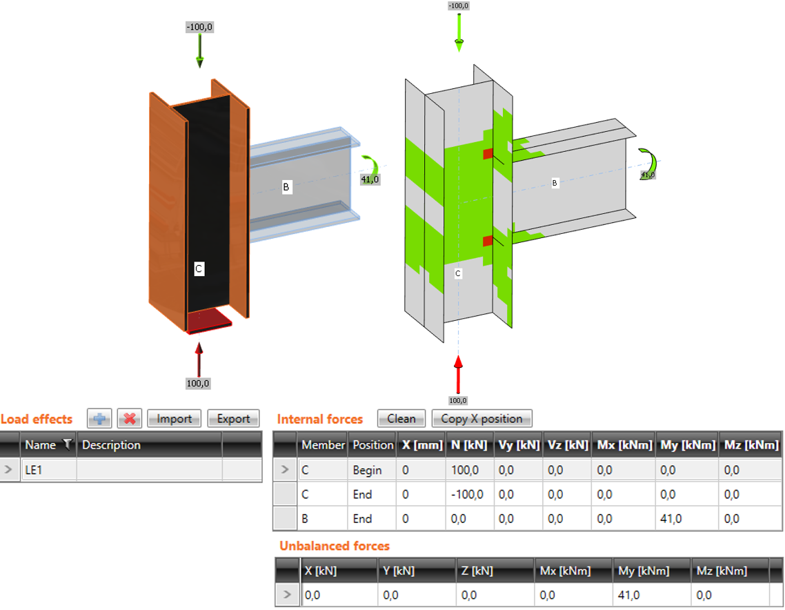
Pokročilé zadání: normálová síla ve sloupu je zohledněna
Zjednodušená metoda je pro uživatele snazší, ale lze ji použít pouze tehdy, když má uživatel zájem o studium prvků přípoje a nikoli o chování celého styčníku.
V případech, kdy je nosný prvek silně zatížen a blízko své mezní únosnosti, je nutný pokročilý režim respektující všechny vnitřní síly ve styčníku.
Koncové síly prvku z modelu rámu jsou přeneseny na konce segmentů prvků. Při přenosu jsou respektovány excentricity prvků způsobené návrhem styčníku.
Analytický model vytvořený metodou CBFEM velmi přesně odpovídá skutečnému styčníku, zatímco analýza vnitřních sil je prováděna na výrazně idealizovaném 3D MKP prutinovém modelu, kde jsou jednotlivé nosníky modelovány pomocí střednicových os a styčníky jsou modelovány pomocí nehmotných uzlů.
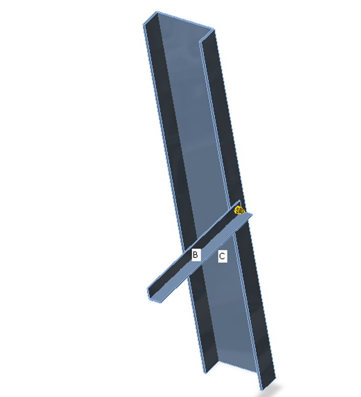
Styčník svislého sloupu a vodorovného nosníku
Vnitřní síly jsou analyzovány pomocí 1D prvků v 3D modelu. Příklad vnitřních sil je znázorněn na následujícím obrázku.
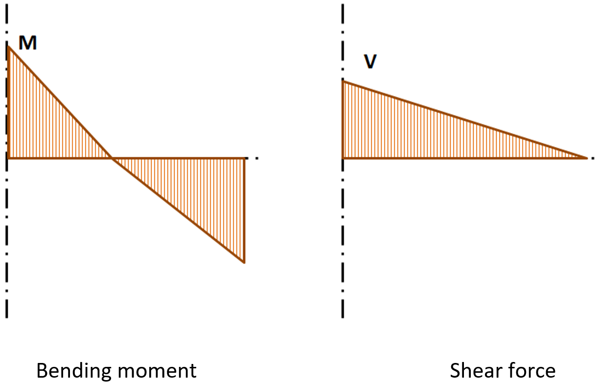
Vnitřní síly ve vodorovném nosníku; M a V jsou koncové síly ve styčníku
Pro návrh styčníku (přípoje) jsou důležité účinky, které prvek vyvozuje na styčník. Tyto účinky jsou znázorněny na následujícím obrázku:
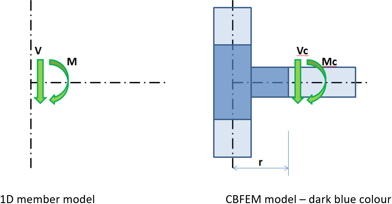
Účinky prvku na styčník; model CBFEM je zobrazen tmavě modrou barvou
Moment M a posouvající síla V působí v teoretickém styčníku. Bod teoretického styčníku v modelu CBFEM neexistuje, a proto zde nelze zatížení aplikovat. Model musí být zatížen účinky M a V, které musí být přeneseny na konec segmentu ve vzdálenosti r
Mc = M – V ∙ r
Vc = V
V modelu CBFEM je koncový průřez segmentu zatížen momentem Mc a silou Vc.
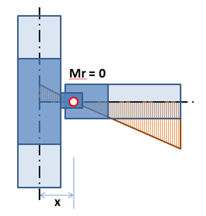
Při návrhu styčníku musí být určena a respektována jeho skutečná poloha vůči teoretickému bodu styčníku. Vnitřní síly v poloze skutečného styčníku se většinou liší od vnitřních sil v teoretickém bodě styčníku. Díky přesnému modelu CBFEM je návrh prováděn na redukované síly – viz moment Mr na následujícím obrázku:
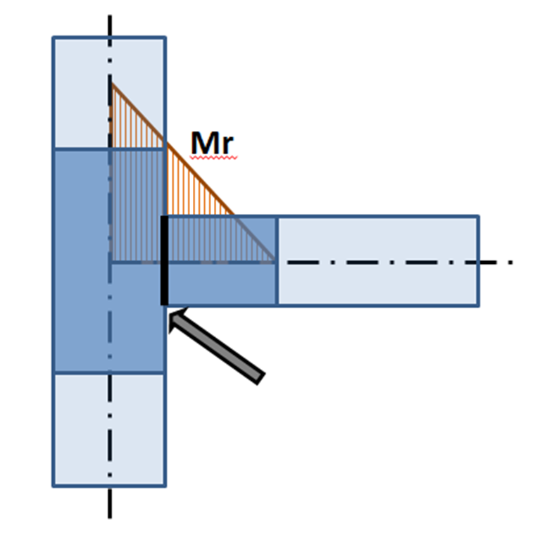
Ohybový moment na modelu CBFEM: šipka ukazuje na skutečnou polohu přípoje
Při zatěžování styčníku musí být respektováno, že řešení skutečného styčníku musí odpovídat teoretickému modelu použitému pro výpočet vnitřních sil. To je splněno pro tuhé styčníky, ale situace může být zcela odlišná pro klouby.
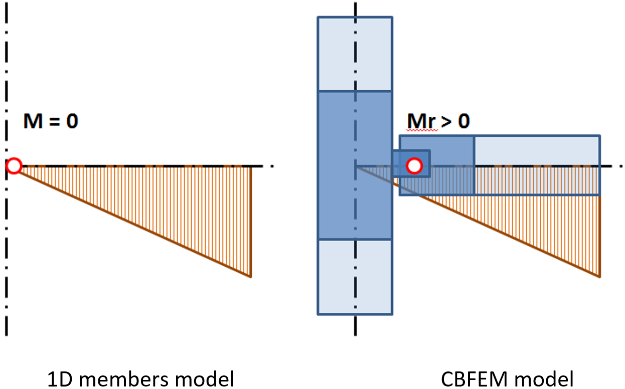
Poloha kloubu v teoretickém 3D MKP modelu a ve skutečné konstrukci
Z předchozího obrázku vyplývá, že poloha kloubu v teoretickém modelu 1D prvků se liší od skutečné polohy v konstrukci. Teoretický model neodpovídá skutečnosti. Při aplikaci vypočtených vnitřních sil je na posunutý styčník aplikován významný ohybový moment a navrhovaný styčník je předimenzovaný nebo jej nelze vůbec navrhnout. Řešení je jednoduché – oba modely musí odpovídat. Buď musí být kloub v modelu 1D prvků definován ve správné poloze, nebo musí být posouvající síla posunuta tak, aby byl moment v poloze kloubu nulový.
Posunutý průběh ohybového momentu na nosníku: nulový moment je v poloze kloubu
Posun posouvající síly lze definovat v tabulce pro zadání vnitřní síly.
Poloha účinku zatížení má velký vliv na správný návrh přípoje. Aby se předešlo veškerým nedorozuměním, umožňujeme uživateli vybrat ze tří možností – Uzel / Šrouby / Poloha.
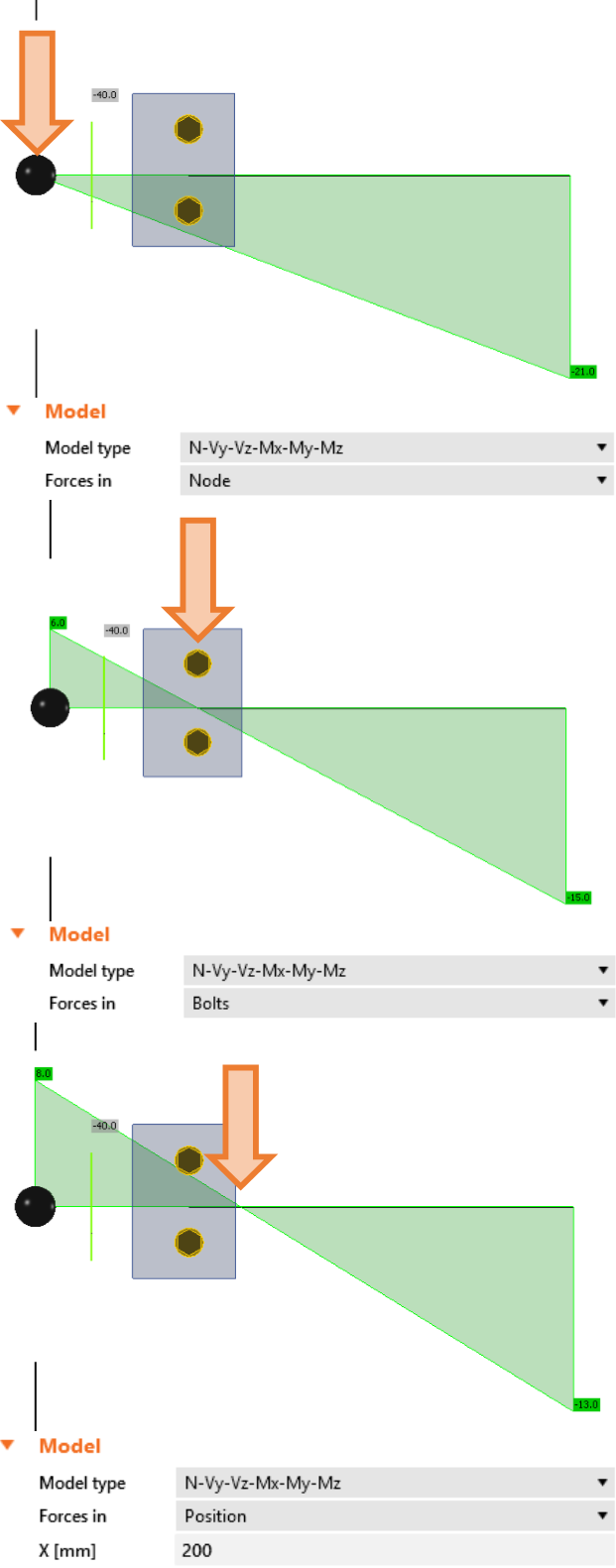
Při výběru možnosti Uzel jsou síly aplikovány na konec vybraného prvku, což je obvykle v teoretickém uzlu, pokud není v geometrii nastaven odsazení vybraného prvku.
Import zatížení z programů MKP
IDEA StatiCa umožňuje import vnitřních sil z programů MKP třetích stran. Programy MKP používají obálku vnitřních sil z kombinací. IDEA StatiCa Connection je program, který řeší ocelový styčník nelineárně (elasticko-plastický materiálový model). Proto nelze použít obálkové kombinace. IDEA StatiCa vyhledává extrémy vnitřních sil (N, Vy, Vz, Mx, My, Mz) ve všech kombinacích na koncích všech prvků připojených ke styčníku. Pro každou takovou extrémní hodnotu jsou použity také všechny ostatní vnitřní síly z dané kombinace ve všech ostatních prvcích. IDEA StatiCa určuje nejhorší kombinaci pro každou komponentu (plech, svar, šroub atd.) v přípoji.
Uživatel může tento seznam zatěžovacích stavů upravit. Může pracovat s kombinacemi v průvodci (nebo BIM), nebo může některé případy přímo smazat v IDEA StatiCa Connection.
Upozornění!
Při importu je nutné zohlednit nevyvážené vnitřní síly. K tomu může dojít v následujících případech:
- Uzlová síla byla aplikována v poloze zkoumaného uzlu. Software nemůže zjistit, který prvek by měl tuto uzlovou sílu přenést, a proto není v analytickém modelu zohledněna. Řešení: Nepoužívejte uzlové síly v globální analýze. V případě potřeby musí být síla ručně přidána k vybranému prvku jako normálová nebo posouvající síla.
- Zatížený neocelový (obvykle dřevěný nebo betonový) prvek je připojen ke zkoumanému uzlu. Takový prvek není v analýze uvažován a jeho vnitřní síly jsou v analýze ignorovány. Řešení: Nahraďte betonový prvek betonovým blokem a kotvením.
- Uzel je součástí desky nebo stěny (obvykle betonové). Deska nebo stěna není součástí modelu a její vnitřní síly jsou ignorovány. Řešení: Nahraďte betonovou desku nebo stěnu betonovým blokem a kotvením.
- Některé prvky jsou ke zkoumanému uzlu připojeny prostřednictvím tuhých vazeb. Takové prvky nejsou zahrnuty v modelu a jejich vnitřní síly jsou ignorovány. Řešení: Přidejte tyto prvky do seznamu připojených prvků ručně.
- V softwaru jsou analyzovány seizmické zatěžovací stavy. Většina programů MKP nabízí modální analýzu pro řešení seizmicity. Výsledky vnitřních sil seizmických zatěžovacích stavů poskytují obvykle pouze obálky vnitřních sil v průřezech. Vzhledem k metodě vyhodnocení (odmocnina součtu čtverců – SRSS) jsou vnitřní síly všechny kladné a není možné najít síly odpovídající vybranému extrému. Není možné dosáhnout rovnováhy vnitřních sil. Řešení: Změňte kladné znaménko některých vnitřních sil ručně.
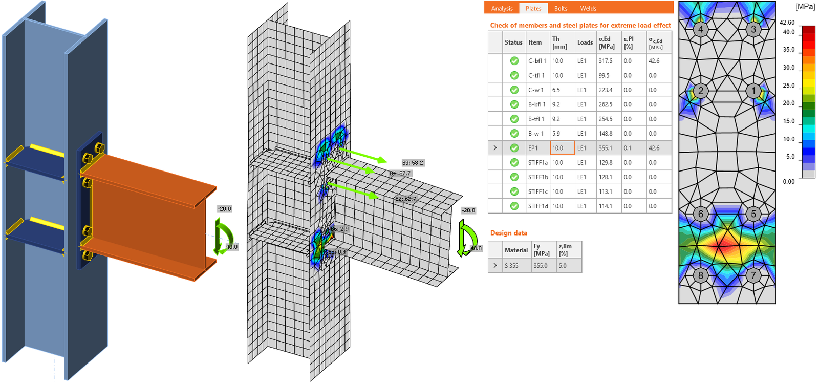
Pevnostní analýza je nejdůležitější analýzou styčníků. Kontroly přetvoření plechů spolu s normovými posouzeními komponent jsou prováděny elasticko-plastickou analýzou.
Analýza styčníků je materiálově nelineární. Přírůstky zatížení jsou aplikovány postupně a hledá se stav napětí. V IDEA StatiCa Connection jsou k dispozici dva volitelné režimy analýzy:
- Odezva konstrukce (styčníku) na celkové zatížení. V tomto režimu je aplikováno veškeré definované zatížení (100 %) a vypočítá se odpovídající stav napětí a deformace.
- Ukončení analýzy při dosažení mezního stavu únosnosti. V nastavení normy by mělo být zaškrtnuto políčko „Stop at limit strain". Stav je nalezen, když plastické přetvoření dosáhne definované meze. V případě, kdy je definované zatížení vyšší než vypočtená únosnost, je analýza označena jako nevyhovující a je vytištěno procento využitého zatížení. Upozorňujeme, že analytická únosnost komponent, například šroubů, může být překročena.
Druhý režim je vhodnější pro praktický návrh. První je vhodný pro podrobnou analýzu složitých styčníků.
Styčníky jsou klasifikovány podle tuhosti jako tuhé, polotuhé a kloubové. Inženýr by měl zajistit, aby tuhost styčníku odpovídala tuhosti nastavené v CAE softwaru. Cílem analýzy tuhosti je získat správné rozdělení zatížení v prvcích a styčnících a správné průhyby prvků a celé konstrukce.
Metoda CBFEM analyzuje tuhost přípoje jednotlivých prvků styčníku. Pro správnou analýzu tuhosti musí být pro každý analyzovaný prvek vytvořen samostatný analytický model. Analýza tuhosti pak není ovlivněna tuhostí ostatních prvků styčníku, ale pouze samotným uzlem a výstavbou přípoje analyzovaného prvku. Zatímco nosný prvek je podepřen pro analýzu únosnosti (prvek SL na obrázku níže), pro analýzu tuhosti jsou podepřeny všechny prvky kromě analyzovaného (viz dva obrázky níže pro analýzu tuhosti prvků B1 a B3). Výjimkou je patní deska sloupu, kde podpory zajišťuje betonový základ; zatížen je pouze analyzovaný prvek a ostatní prvky mají omezení pouze podle jejich typu modelu.
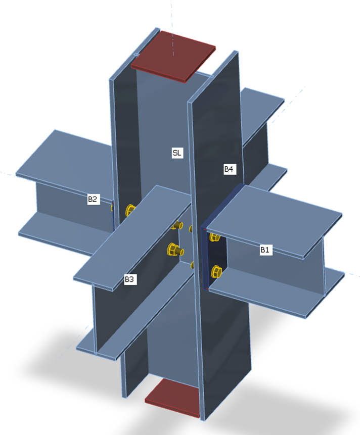
Podpory na prvcích pro analýzu únosnosti
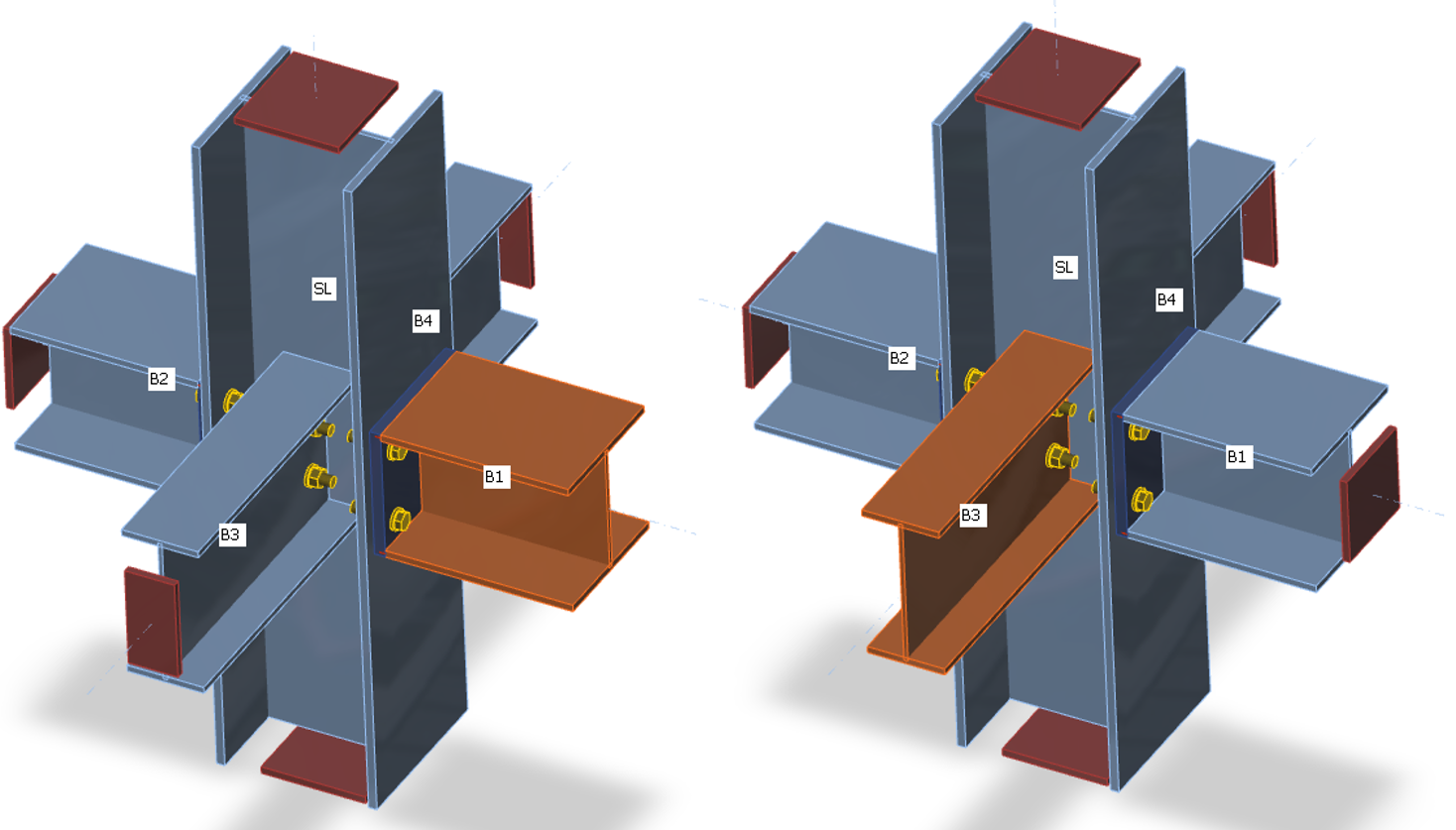
| Podpory na prvcích pro analýzu tuhosti prvku B1 | Podpory na prvcích pro analýzu tuhosti prvku B3 |
Zatížení lze přikládat pouze na analyzovaný prvek. Je-li definován ohybový moment My, analyzuje se rotační tuhost kolem osy y. Je-li definován ohybový moment Mz, analyzuje se rotační tuhost kolem osy z. Je-li definována normálová síla N, analyzuje se osová tuhost přípoje.
Křivka moment–rotace (nebo zatížení–deformace) se vypočítá pro dva modely:
- Úplný model přípoje – s prvky, plechy, šrouby, svary atd. (materiálově nelineární analýza)
- Model prvku – pouze s prvky tuhle spojenými v uzlu (lineárně elastická analýza)
Zobrazený diagram vznikne odečtením modelu prvku od úplného modelu přípoje. Tímto způsobem je vyloučena elastická deformace prvků, která je již zahrnuta v modelu celé konstrukce.
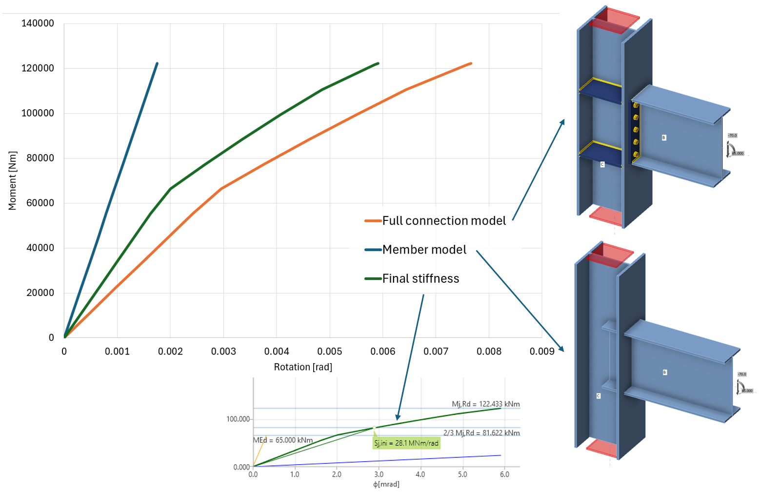
Program generuje úplný diagram automaticky; je přímo zobrazen v grafickém rozhraní a lze jej přidat do výstupní zprávy. Rotační nebo osová tuhost může být studována pro konkrétní návrhová zatížení. IDEA StatiCa Connection dokáže také pracovat s interakcí ostatních vnitřních sil.
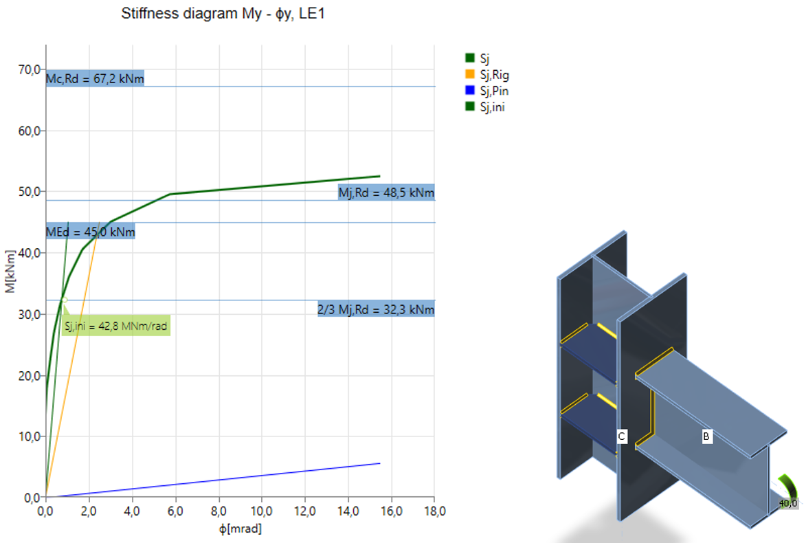
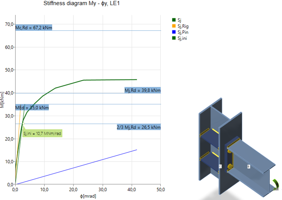
Diagram zobrazuje:
- Úroveň návrhového zatížení MEd
- Limitní hodnotu únosnosti přípoje pro 5% ekvivalentní přetvoření Mj,Rd; limit pro plastické přetvoření lze změnit v nastavení normy
- Limitní hodnotu únosnosti připojeného prvku (užitečné také pro seizmický návrh) Mc,Rd
- 2/3 limitní únosnosti pro výpočet počáteční tuhosti
- Hodnotu počáteční tuhosti Sj,ini
- Hodnotu sečnové tuhosti Sjs
- Limity pro klasifikaci přípoje – tuhý a kloubový
- Rotační deformaci Φ
- Rotační kapacitu Φc
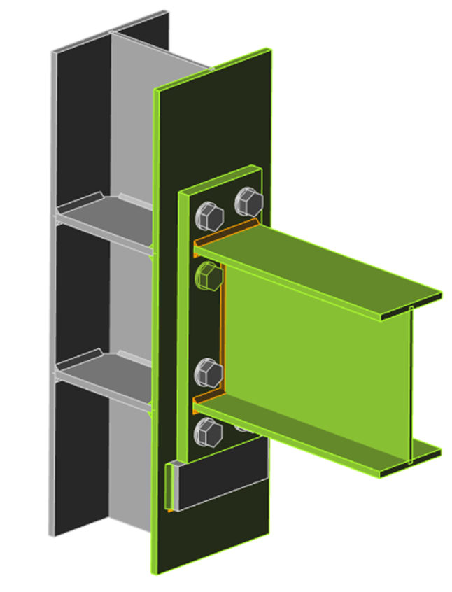
Tuhý svařovaný přípoj
Polotuhý šroubovaný přípoj
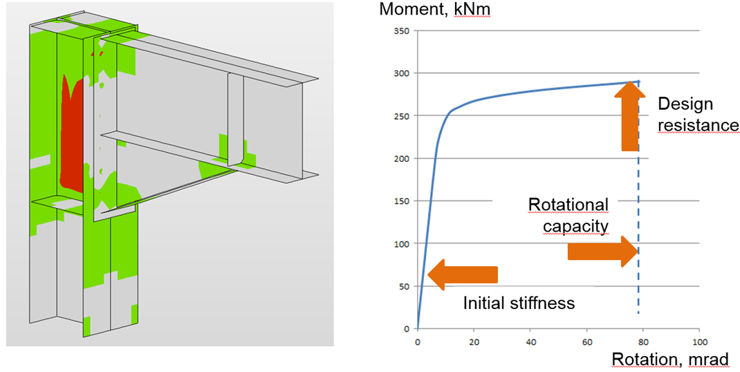
Po dosažení 5% přetvoření ve stojině sloupu při smyku se plastické zóny rychle šíří
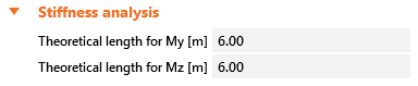
Styčník je klasifikován podle tuhosti do kategorie tuhý, polotuhý nebo kloubový podle příslušné normy. Pro analyzovaný prvek lze nastavit teoretickou délku prvku:
Jak se přikládají zatížení?
V analýze tuhosti je zatížen a vyšetřován pouze jeden prvek. Analyzovaný prvek může být zatížen:
- Normálovou silou N
- Posouvajícími silami Vy a Vz
- Ohybovými momenty My a Mz
- Kroucením Mx
Všechny účinky zatížení jsou přikládány současně. Jsou-li přiložená zatížení příliš malá, jsou všechna zvýšena součinitelem tak, aby bylo dosaženo únosnosti styčníku (přiložené síly musí být větší než 1). Při vytváření diagramů moment–rotace nebo zatížení–deformace jsou všechny účinky zatížení zvyšovány postupně proporcionálně.
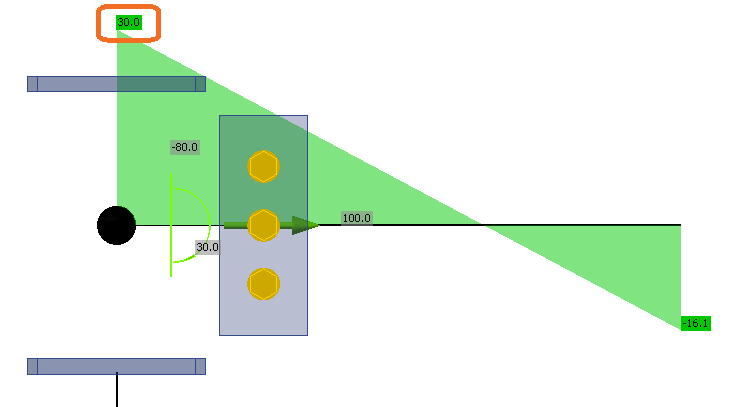
Například analyzovaný prvek je zatížen:
- Normálovou silou N = 50 kN
- Posouvající silou Vz = -80 kN
- Ohybovým momentem My = 30 kNm
Únosnosti prvku jsou:
- Normálová únosnost NR = 2 111 kN
- Smyková únosnost Vz,R = 763 kN
- Únosnost v ohybovém momentu My,R = 226 kNm
Zatížení jsou násobena součinitelem:
Poznámka: pokud posouvající síla není přiložena v uzlu, tj. působí na rameni, je ovlivněn ohybový moment. Jako zadané zatížení se používá ohybový moment v uzlu, jak je patrné z drátového modelu.
V tomto příkladu je součinitel . Zadaná zatížení jsou násobena a poté přikládána postupně, přičemž výsledky jsou vynášeny do diagramu tuhosti. Přiložená zatížení jsou rozdělena do 12 kroků a při přibližování se k únosnosti přípoje jsou kroky dále zjemňovány. Příklad prvních tří kroků je uveden v následující tabulce:
| Zadaná zatížení | Přiložená zatížení | První krok | Druhý krok | Třetí krok | |
| 100% | 8,33% | 16,67% | 25,00% | ||
| N | 50 | 377 | 31 | 63 | 94 |
| Vy | 0 | 0 | 0 | 0 | 0 |
| Vz | -80 | -603 | -50 | -100 | -151 |
| Mx | 0 | 0 | 0 | 0 | 0 |
| My | 30 | 226 | 19 | 38 | 57 |
| Mz | 0 | 0 | 0 | 0 | 0 |
Deformační kapacita
Deformační kapacita/duktilita δCd patří spolu s únosností a tuhostí ke třem základním parametrům popisujícím chování přípojů. U momentových přípojů je duktilita zajištěna dostatečnou rotační kapacitou φCd. Deformační/rotační kapacita se vypočítává pro každý přípoj ve styčníku samostatně.
Software odhaduje deformační kapacitu jako bod, ve kterém je dosažena jedna z následujících podmínek:
- Je dosažena únosnost šroubu nebo kotvy v tahu, smyku nebo interakci tah/smyk
- Je dosažena únosnost svaru
- Plastické přetvoření v pleších dosahuje 15 %
Odhad rotační kapacity je důležitý u přípojů vystavených seizmickému zatížení, viz Gioncu a Mazzolani (2002) a Grecea (2004), a extrémnímu zatížení, viz Sherbourne a Bahaari (1994 a 1996). Deformační kapacita komponent je studována od konce minulého století (Foley a Vinnakota, 1995). Faella et al. (2000) provedli zkoušky na T-prvcích a odvodili analytické výrazy pro deformační kapacitu. Kuhlmann a Kuhnemund (2000) provedli zkoušky na stojině sloupu vystavené příčnému tlaku při různých úrovních tlakové normálové síly ve sloupu. Da Silva et al. (2002) předpověděli deformační kapacitu při různých úrovních normálové síly v připojeném prvku. Na základě výsledků zkoušek v kombinaci s analýzou metodou konečných prvků byly analytickými modely stanoveny deformační kapacity základních komponent (Beg et al., 2004). V této práci jsou komponenty reprezentovány nelineárními pružinami a vhodně kombinovány za účelem stanovení rotační kapacity styčníku pro přípoje s čelní deskou – s prodlouženou nebo zarovnanou čelní deskou – a svařované přípoje. Pro tyto přípoje byly jako nejdůležitější komponenty, které mohou významně přispívat k rotační kapacitě, identifikovány: stojina v tlaku, stojina sloupu v tahu, stojina sloupu ve smyku, pásnice sloupu v ohybu a čelní deska v ohybu. Komponenty vztahující se ke stojině sloupu jsou relevantní pouze tehdy, pokud ve sloupu nejsou výztuhy odolávající tlakovým, tahovým nebo smykovým silám. Přítomnost výztuhy eliminuje příslušnou komponentu a její příspěvek k rotační kapacitě styčníku lze proto zanedbat. Čelní desky a pásnice sloupu jsou důležité pouze u přípojů s čelní deskou, kde komponenty působí jako T-prvek, přičemž je zahrnuta také deformační kapacita šroubů v tahu. Otázky a limity deformační kapacity přípojů z vysokopevnostní oceli studovali Girao et al. (2004).
Návrh únosnosti je součástí posouzení styčníku při seismickém návrhu. Při využití duktility konstrukce musí být proveden návrh únosnosti.
Cílem návrhu únosnosti je potvrdit, že budova vykazuje řízené duktilní chování, aby nedošlo k jejímu zřícení při seismickém zatížení na návrhové úrovni.
Disipativní prvek je vybrán se zvýšenou únosností a upraveným materiálovým diagramem. Součinitel přepevnosti je definován v materiálech a součinitel deformačního zpevnění je definován v operaci disipativního prvku. Upozorňujeme, že názvosloví se mezi normami liší. Disipativní prvek je vyloučen z posouzení přetvoření plechů.
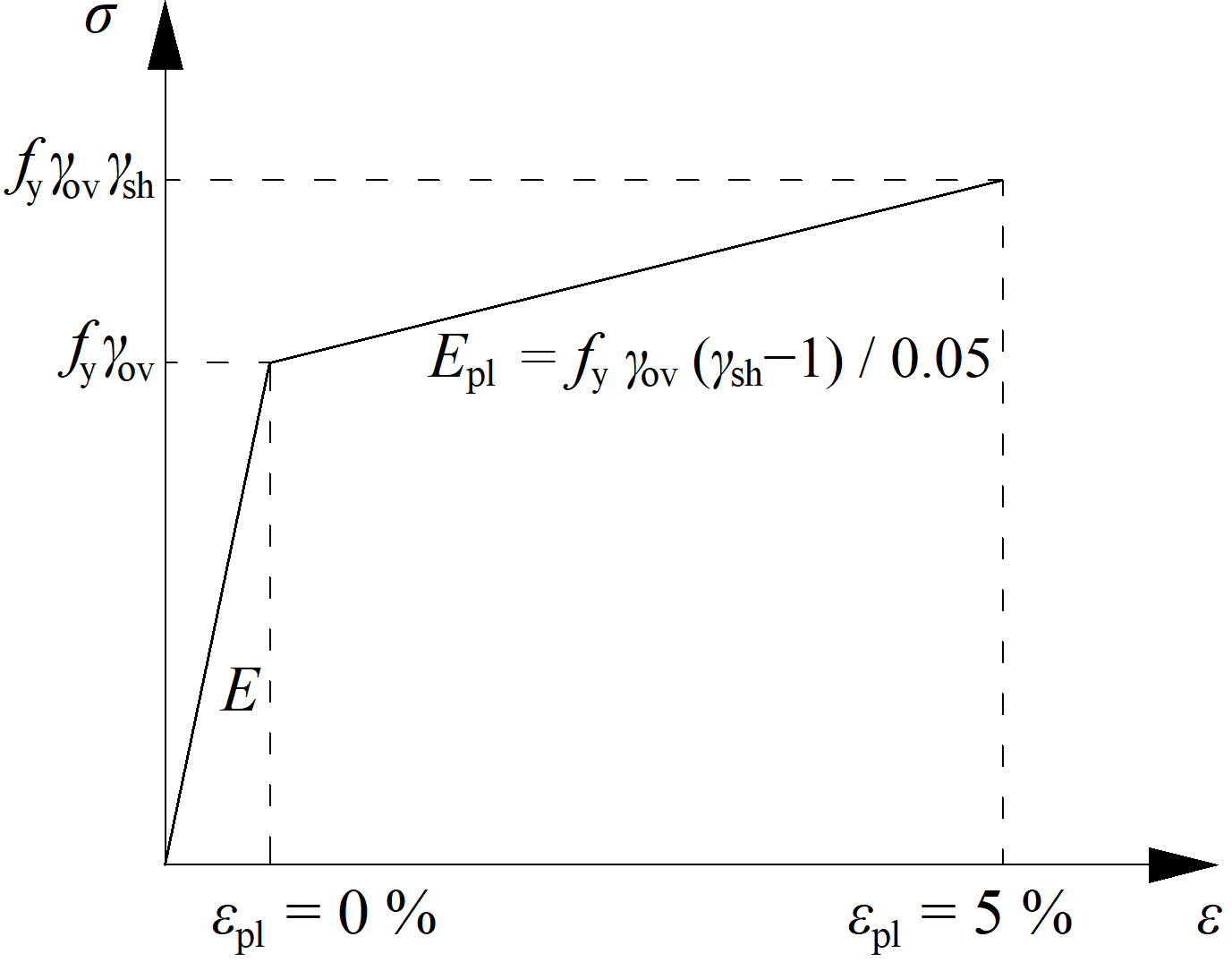
Upravený materiálový diagram pro disipativní prvek
IDEA StatiCa Connection posuzuje přípoj na přiložené návrhové zatížení, které by mělo vytvořit plastický kloub ve vybraném disipativním prvku, obvykle v nosníku. Plastické přetvoření v disipativním prvku by mělo být přibližně 5 %. To může sloužit jako potvrzení, že velikost a poloha zatížení byly stanoveny správně.
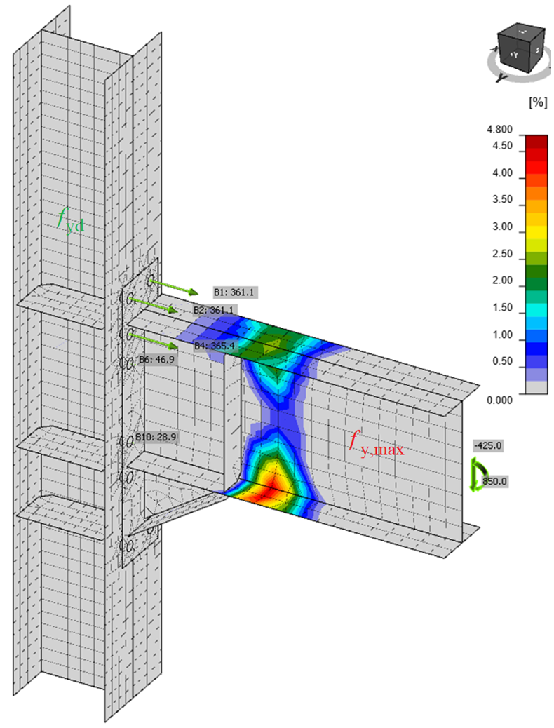
Plastický kloub vytvořený na zamýšleném místě disipativního prvku – nosníku
Podpory spojitého prvku jsou automaticky definovány jako podepřené na jednom konci a s vetknutými momenty na druhém konci. Tímto způsobem může být spojitý sloup zatížen normálovou silou a posouvajícími silami a zároveň se jedna strana může posunout do strany, čímž se odhalí porušení stojiny sloupu smykem.
Upozorňujeme, že konstrukční zásady jsou velmi důležité pro seismicky odolné styčníky, ale nejsou v IDEA StatiCa posuzovány.
Návrhář obvykle řeší úlohu návrhu přípoje/styčníku pro přenos známého návrhového zatížení. Je však také užitečné vědět, jak daleko je návrh od mezního stavu, tj. jak velká je rezerva v návrhu a jak je bezpečný. Toho lze jednoduše dosáhnout pomocí typu analýzy – Návrhová únosnost styčníku.
Uživatel zadá návrhové zatížení stejně jako při standardním návrhu. Software automaticky proporcionálně zvyšuje všechny složky zatížení, dokud některý ze zahrnutých posouzení nevyhoví.
Analýzy DR provádějí posouzení následujících komponent:
- Plastické přetvoření v plechách
- Šrouby – smyk, tah a kombinace tahu a smyku
- Kotvy – tahová a smyková ocelová únosnost
- Svary
Upozorňujeme, že ostatní komponenty nezahrnuté ve výše uvedeném seznamu nebudou posouzeny z důvodu neznámých směrů sil v komponentách. Z tohoto důvodu by měla být vždy provedena analýza EPS, aby bylo zajištěno správné provedení všech posouzení.
Uživatel získá poměr maximálního zatížení k návrhovému zatížení. Je také poskytnut jednoduchý diagram.
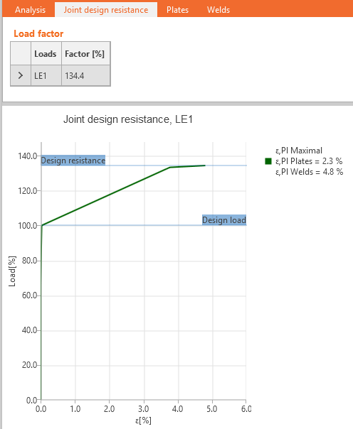
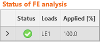
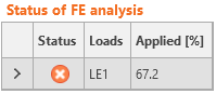
Výsledky uživatelem definovaných zatěžovacích stavů jsou zobrazeny, pokud není faktor návrhové únosnosti styčníku menší než 100 %, což by znamenalo, že výpočet nekonvergoval a je zobrazen poslední konvergovaný krok zatěžovacího stavu.
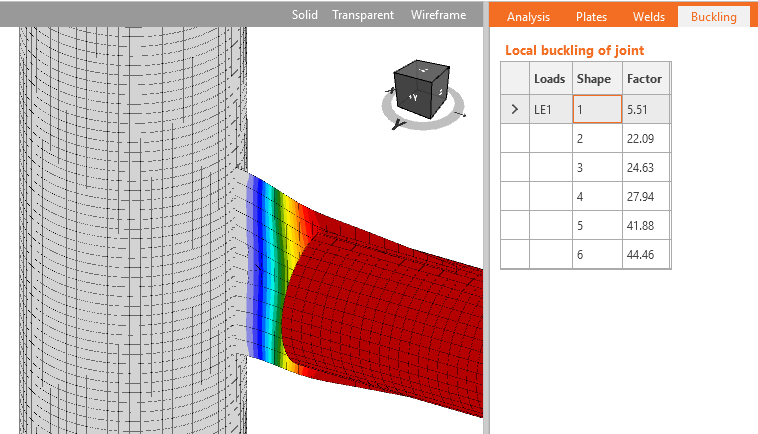
Boulení obvykle není v styčnících zásadním problémem. Přesto je třeba ověřit, že nedochází k problémům s boulením a že výsledky analýzy únosnosti, která využívá pouze geometricky lineární analýzu, jsou správné.
IDEA StatiCa Connection může provést lineární analýzu boulení modelu styčníku. Výsledky jsou prezentovány ve formě tvarů boulení. Pro každý tvar boulení je vypočteno kritické zatížení, při němž dochází k boulení dokonalého modelu. Kritické zatížení je vyjádřeno násobiteli zatížení působícího na styčník. Na základě tvaru boulení a násobitele kritického zatížení může uživatel stanovit bezpečný návrh z hlediska boulení.
Některé normy, např. Eurocode (EN 1993-1-1, kapitola 5.2.1), doporučují násobitel kritického zatížení vyšší než 15 pro prutové modely konstrukcí. Pokud je násobitel kritického zatížení vyšší než 15, norma nevyžaduje posouzení boulení prvků.
U styčníků je situace odlišná a norma neposkytuje žádné konkrétní doporučení. Návrh z hlediska lokálního boulení musí být řešen jiným způsobem. Obecně lze lokální boulení rozdělit do tří skupin:
- Plechy spojující jednotlivé prvky
- Výztužné plechy ve styčníku – výztuhy, žebra, krátké náběhy
- Uzavřené průřezy a tenkostěnné průřezy
Boulení plechů ze skupiny 1 ovlivňuje tvar boulení celého prvku. Proto se doporučuje aplikovat na tyto plechy stejná pravidla jako pro tyto prvky, tj. uvažovat bezpečný násobitel kritického zatížení 15 a vyšší. Inženýr by měl ověřit, že skutečné provedení styčníku odpovídá okrajovým podmínkám modelu použitého pro analýzu boulení celé konstrukce.
Plechy ze skupiny 2 ovlivňují lokální boulení styčníku. Pro takové plechy je bezpečná hranice násobitele kritického zatížení 15 konzervativní, ale konkrétní pokyny v normách chybí. Pokyny poskytují výzkumné práce doporučující bezpečnou hranici násobitele kritického zatížení rovnou 3.
Boulení plechů a prvků ze skupiny 3 je velmi problematické a je nutné individuální posouzení každého konkrétního případu.
Pro plechy s násobitelem kritického zatížení menším než doporučené hodnoty (15 pro skupinu 1, 3 pro skupinu 2) nelze použít plastický návrh. V takovém případě jsou pro návrh přípoje vyžadovány jiné metody:
- Normové posouzení podle příslušné návrhové normy, např. Eurocode nebo AISC Specification nebo Design Manual
- Obecná metoda podle EN 1993-1-5 příloha B – Prvky s proměnným průřezem, kde jsou výsledky MNA a LBA využity ke stanovení únosnosti při boulení štíhlých plechů
- Geometricky a materiálově nelineární analýza s imperfekcemi dostupná v aplikaci IDEA StatiCa Member
Výsledek lineární analýzy boulení v IDEA StatiCa Connection není definitivním posouzením. Normy neposkytují dostatečné pokyny. Posouzení vyžaduje inženýrský úsudek a IDEA StatiCa poskytuje jedinečné nástroje, které nejsou dostupné ve standardním návrhových softwaru.
Styčníkový plech jako prodloužení příhradového nosníku – příklad plechu ze skupiny 1, u kterého lze boulení zanedbat, pokud je kritický součinitel boulení vyšší než 15
Příklady tvarů boulení plechů ze skupiny 2, u nichž lze boulení zanedbat, pokud je kritický součinitel boulení vyšší než 3
Model použitý pro analýzu boulení je podepřen jinými podporami, než jaké nastavil uživatel v typu analýzy napětí a přetvoření (EPS). Nosný prvek zůstává plně podepřen. Typ modelu nosníku nastaveného jako N-Vy-Vz-Mx-My-Mz (volný pohyb v typu analýzy napětí a přetvoření) je v analýze boulení plně podepřen. Všechny ostatní typy analýzy nosníku mají zamezené ohybové momenty a normálovou sílu, ale jsou volné pro boční pohyb.
- Typ modelu N-Vy-Vz-Mx-My-Mz: podpory v modelu boulení: N-Vy-Vz-Mx-My-Mz
- Typ modelu N-Vy-Vz: podpory v modelu boulení: N-Mx-My-Mz
- Typ modelu N-Vz-My: podpory v modelu boulení: N-Mx-My-Mz
- Typ modelu N-Vy-Mz: podpory v modelu boulení: N-Mx-My-Mz
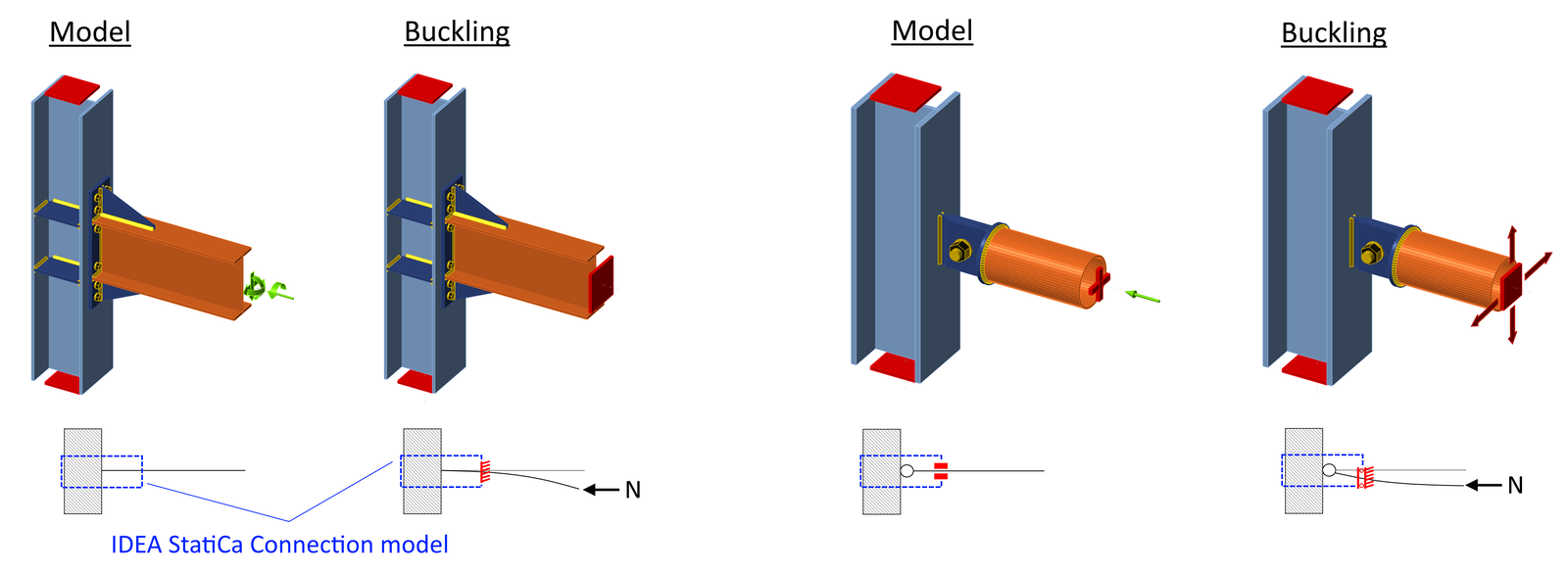
Předpokládá se, že v případě tuhého styčníku uživatel zadává ohybový moment a boulení krátkého segmentu nosníku není relevantní. Na druhé straně, v případě kloubového styčníku uživatel zadává pouze normálovou a smykovou sílu bez ohybového momentu, ale boulení kloubového prvku je relevantní, a proto přispívá k součiniteli boulení. Viz obrázek níže. „Model" zobrazuje model v typu analýzy napětí-přetvoření a „Boulení" zobrazuje model v analýze boulení.
Analýza metodou konečných prvků nemusí konvergovat z několika důvodů, obvykle kvůli prvku, který není dostatečně podepřen a může se volně pohybovat nebo otáčet.
Analýza metodou konečných prvků vyžaduje mírně rostoucí diagram napětí-přetvoření materiálových modelů. V některých případech složitých modelů, např. s více kontakty, může zvýšení počtu divergentních iterací pomoci s konvergencí. Tuto hodnotu lze nastavit v nastavení normy. Nejčastějšími příčinami selhání analýzy jsou singularity, kdy části modelu nejsou správně propojeny a mohou se volně pohybovat nebo otáčet. Uživatel je upozorněn a měl by zkontrolovat model na chybějící svary nebo šrouby. Deformovaný tvar je zobrazen s prvky, které způsobily první singularitu, posunutými o 1 m, aby bylo možné singularitu snadno odhalit.
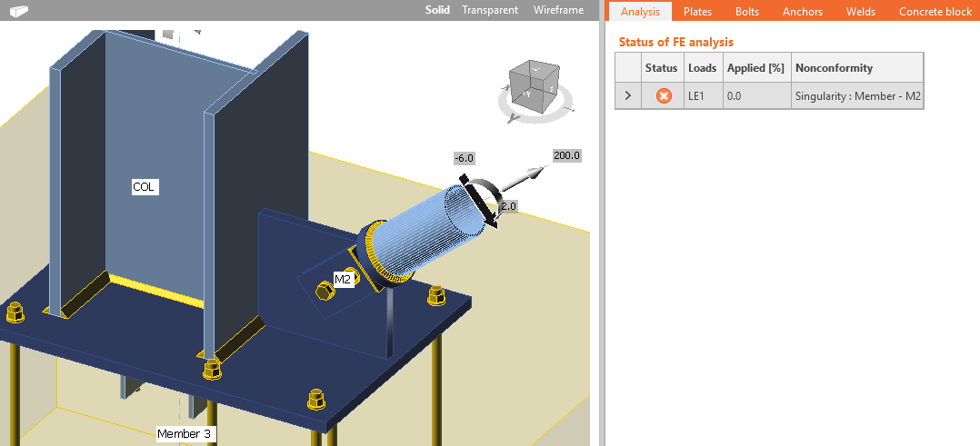
Chybějící svary na styčníkových pleších vedoucí k singularitě
Ocelovo-dřevěné přípoje jsou v současné době určeny pouze pro posouzení ocelových plechů a stanovení vektorů sil ve spojovacích prvcích. Styčníkové plechy lze použít jako uzavřené nebo vložené.
Materiálové vlastnosti dřeva nejsou specifikovány. Posouzení spojovacích prvků a dřeva je třeba provést ručně nebo v jiném softwaru podle příslušných návrhových pravidel. Proto není k dispozici analýza tuhosti.
Posouzení ostatních komponent ocelových přípojů je prováděno normovým posouzením standardním způsobem.
Více informací o práci s ocelovo-dřevěnými přípoji naleznete v článku znalostní báze.
IDEA StatiCa Connection pro návrh styčníků tenkostěnných prvků by měl být ponechán pouze zkušeným inženýrům. Analýza boulení je nezbytná a každý tvar vlastního tvaru musí být pečlivě analyzován.
Software IDEA StatiCa Connection je určen pro posouzení přípojů válcovaných prvků, které nejsou výrazně ovlivněny boulením. Geometricky lineární a materiálově nelineární analýza je prováděna z důvodu rychlého a stabilního výpočtu. Tato analýza však není dostatečná pro ztrátu stability. Pokud může být boulení problémem, provedení lineární analýzy boulení pomáhá odhalit nebezpečná místa a poskytnout součinitel pro Eulerův bod bifurkace, ale to stále nestačí pro tenkostěnné prvky. Pro tenkostěnné prvky je vhodná pouze geometricky nelineární analýza s imperfekcemi.
Pokud se uživatel přesto rozhodne použít software IDEA StatiCa Connection pro posouzení přípojů tenkostěnných prvků, měl by:
- Provést lineární analýzu boulení a pečlivě vyhodnotit každý tvar boulení; prvních 5 prezentovaných tvarů boulení nemusí být dostatečných (Jak zvýšit počet vyhodnocovaných tvarů)
- Nespoléhat na plasticitu ocelových plechů a raději omezit napětí von Mises na mez kluzu nebo i nižší hodnotu
- Mít na paměti, že lokální boulení, které není uvažováno, může přerozdělit vnitřní síly v komponentách odlišným způsobem
- Mít na paměti, že tuhost komponent může být odlišná v důsledku různých způsobů porušení nebo jejich kombinace.
- Mít na paměti, že prezentovaná posouzení a konstrukční zásady komponent (např. šrouby, svary) jsou vodítky pro standardní prvky. Posouzení pro tenkostěnné prvky se mohou lišit, a v takovém případě poskytnutá posouzení nejsou správná.
Návrh přípojů tenkostěnných prvků je velmi specifický pro každý případ a nelze poskytnout žádné obecné vodítko. IDEA StatiCa Connection nebyl pro toto použití validován.
Posouzení komponent – EN
V EN 1993-1-1 jsou tenkostěnné prvky definovány jako: „Průřezy třídy 4 jsou ty, u nichž dojde k lokálnímu boulení dříve, než je dosaženo meze kluzu v jedné nebo více částech průřezu." Hlavní část Eurokódu pro ocel je omezena na prvky s tloušťkou materiálu t ≥ 3 mm. Kapitola 4 – Svarové přípoje se vztahuje pouze na tloušťku materiálu t ≥ 4 mm. Posouzení komponent poskytovaná softwarem se proto nevztahují na za studena tvarované prvky s menšími tloušťkami. Uživatelé by si toho měli být vědomi a nahradit posouzení příslušnými vzorci z EN 1993-1-3 ručně.
Analýza styčníků dutých průřezů by měla být rovněž pečlivě provedena pro prvky, které jsou mimo rozsah platnosti pro svarové styčníky – EN 1993-1-8 – Tabulka 7.1. Pro takové styčníky neexistují žádná vodítka a výsledky softwaru nebyly validovány.
Posouzení komponent – AISC
V kapitole A normy AISC 360-16 je uvedena poznámka pro uživatele: „Pro návrh za studena tvarovaných ocelových konstrukčních prvků se doporučují ustanovení severoamerické specifikace AISI pro návrh za studena tvarovaných ocelových konstrukčních prvků (AISI S100), s výjimkou za studena tvarovaných dutých konstrukčních průřezů (HSS), které jsou navrhovány v souladu s touto specifikací." AISI S100 a AS/NZS 4600 poskytují vzorce pro stanovení smykové a tahové únosnosti nejběžnějších typů spojovacích prvků spolu s jejich rozsahem použití.
Posouzení komponent – CISC
CSA S16-14 uvádí v kapitole 1: „Požadavky na ocelové konstrukce, jako jsou mosty, stožáry antén, offshore konstrukce a za studena tvarované ocelové konstrukční prvky, jsou uvedeny v jiných normách skupiny CSA."
Popis modelu
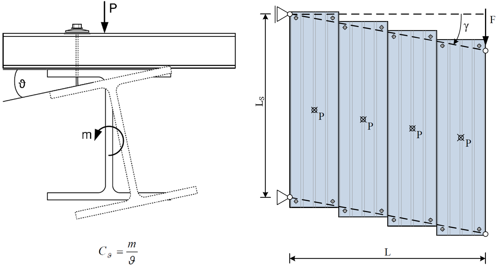
Lateral-torsional restraint je simulováno dvěma tuhostmi přidanými k libovolnému plechu:
- Boční (smyková) S [N] působící ve směru osy y lokálního souřadnicového systému plechu
- Torzní C [Nm/m] působící kolem osy x lokálního souřadnicového systému plechu
Uživatelé mohou vybrat libovolný plech prvku, délku zajištění, typ (spojitý nebo diskrétní s nastavenou roztečí) a boční a torzní tuhosti.
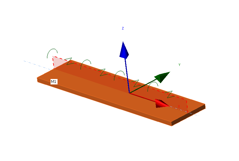
Lokální souřadnicový systém plechu s aplikovaným LTR
Uzly konečných prvků jsou propojeny podél šířky plechu tuhými prvky typu 3 (RBE3) do jednoho bodu na podélné ose plechu. Torzní tuhost je v tomto bodě aplikována speciálním prvkem s jedinou tuhostí – otočením kolem osy x. Tento bod je také propojen dvěma dalšími RBE3 se speciálním prvkem mezi nimi s jednou tuhostí – posunem ve směru osy y.
Boční tuhost je uživatelem nastavena jako volná, tuhá nebo s definovanou hodnotou tuhosti. Tuhá tuhost je dostatečně vysoká, nastavena jako 1000násobek smykové tuhosti plechu. Tuhost je zadána na jednotku délky (jeden metr) s jednotkou síly [N]. Tuhost jednoho prvku má jednotku síly dělenou jednotkou délky [N/m] a je pak:
kde:
- – vzdálenost mezi dvěma body [m]
Pro diskrétní typ je rozteč nastavena přímo uživatelem. Pro spojitý typ je rozteč dostatečně malá, aby chování plechu nebylo roztečí ovlivněno.
Obdobně je torzní tuhost uživatelem nastavena jako volná, tuhá nebo s definovanou hodnotou tuhosti. Tuhá tuhost je dostatečně vysoká, nastavena jako 1 000násobek ohybové tuhosti plechu. Tuhost je zadána na jednotku délky (jeden metr) s jednotkou ohybového momentu dělenou jednotkou délky [Nm/m]. Tuhost jednoho prvku má jednotku ohybového momentu dělenou druhou mocninou jednotky délky [Nm/m2] a je pak:
Pro lepší pochopení hodnot tuhostí viz dokument European Recommendations on the Stabilization of Steel Structures by Sandwich Panels.
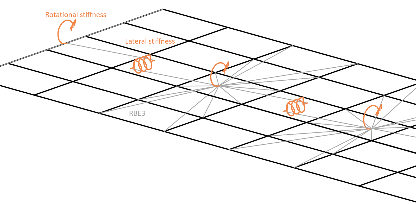
Skryté konečné prvky a RBE3 zajišťují boční a torzní tuhost plechu prvku
Poznámka: RBE3 jsou pouze interpolační vazby, které samy o sobě neposkytují žádnou tuhost.
Ověření
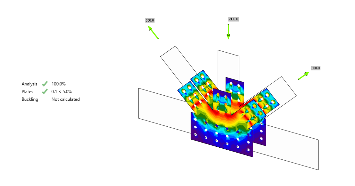
Model poskytující LTR byl ověřen softwarem LTBeam, který využívá prutové (1D) prvky se sedmi stupni volnosti. To znamená, že průřez se nedeformuje, ale prvek dokáže zachytit kroucení. Porovnání je ukázáno na příkladu průřezu IPE 180 z oceli třídy S355 s délkou 6 m. Nosník je na obou koncích vetknut a zatížen rovnoměrným zatížením 20 kN/m působícím na horní pásnici. Software LTBeam je schopen stanovit elastický kritický moment odpovídající výsledku lineární analýzy boulení (LBA) v IDEA StatiCa Member.
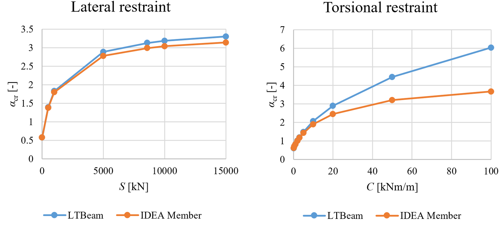
Porovnání LTBeam a IDEA StatiCa Member pro boční a torzní tuhost
Součinitel kritického zatížení při elastickém boulení s boční tuhostí je podle obou softwarů velmi podobný. Mezní boční tuhost, při níž má klopení vliv nejvýše 5 % na ohybovou únosnost nosníku, se vypočítá podle EN 1993-1-1 jako Slim = 8 589 kN. Výsledky s torzním zajištěním se však při vyšších hodnotách rotační tuhosti rozcházejí. Při sledování deformovaného tvaru v IDEA StatiCa Member je rozdíl způsoben deformací průřezu, kterou lze zachytit pouze skořepinovým modelem. LTBeam poskytuje nerealisticky vysoké součinitele kritického zatížení při vysoké torzní tuhosti.
Pro ověření tohoto tvrzení byl na ETH university vytvořen skořepinový model v programu ABAQUS. Nosník je opět vetknut na obou koncích, zhotoven z oceli třídy S355 a má délku 6 m. Byl použit průřez nosníku IPE 240. Mezní torzní tuhost, tj. klopení má vliv nejvýše 5 % na ohybovou únosnost nosníku, byla vypočtena jako Clim = 27,13 kNm/m. Model je zatížen silou uprostřed rozpětí na horní pásnici.
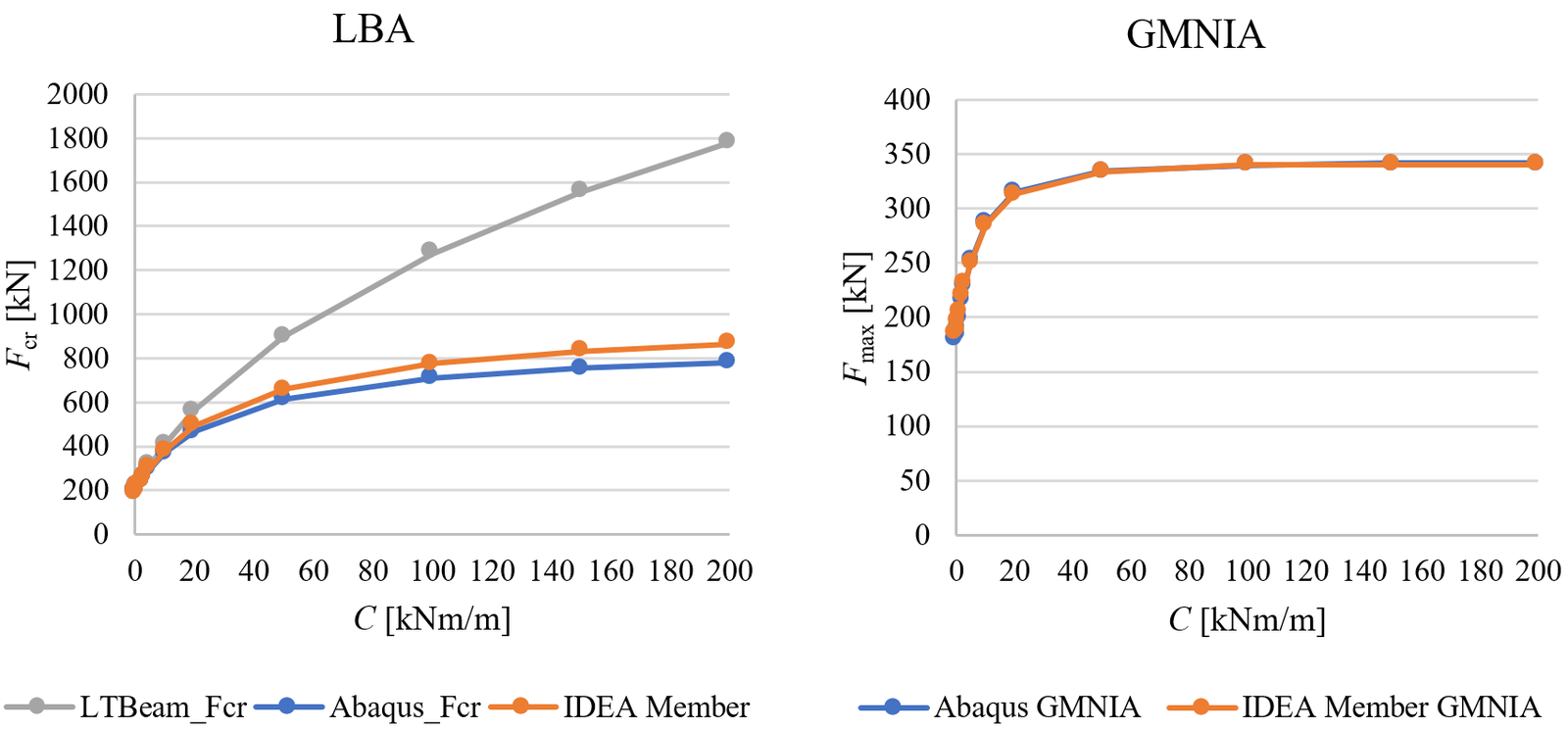
Porovnání ABAQUS, LTBeam a IDEA StatiCa Member pro torzní tuhost
Vliv torzní tuhosti je v obou skořepinových modelech velmi podobný a LTBeam se odchyluje. Nejdůležitější je, že únosnosti při boulení stanovené metodou GMNIA v ABAQUS a IDEA StatiCa Member se téměř shodují – rozdíly jsou do 4 %.
Odhad tuhostí
LTR zajištěné podlahami vyplněnými betonem se spřažením pomocí spřahovacích trnů lze považovat za tuhé přinejmenším v případě boční tuhosti. Tuhosti poskytované trapézovými plechy sendvičových panelů jsou výrazně nižší a lze je stanovit experimentálně nebo výpočtem. Nejčastěji budou hodnoty boční a torzní tuhosti doporučeny výrobci sendvičových panelů nebo jiných typů opláštění.
Výpočet boční tuhosti S [N] poskytované trapézovými plechy je uveden v EN 1993-1-3, kapitola 10:
kde:
- t – návrhová tloušťka trapézového plechu [mm]
- broof – šířka střechy, tj. pro sedlovou střechu vzdálenost mezi hřebenem a okapem [mm]
- s – vzdálenost mezi nosníky [mm]
- hw – výška profilu trapézového plechu [mm]
Vzorec platí, pokud je trapézový plech připojen k nosníku v každém žebru. Pokud je plech připojen k nosníku pouze v každém druhém žebru, je třeba nahradit S hodnotou 0,2 S.
Boční tuhost sendvičových panelů je popsána v doporučení ECCS. Klíčová je tuhost spojovacích prvků:
kde:
- kv – smyková tuhost upevnění
- B – šířka sendvičového panelu
- nk – počet párů spojovacích prvků na panel a podporu
- ck – vzdálenost mezi dvěma spojovacími prvky páru
Torzní tuhost je složitější a lze ji také odhadnout pomocí doporučení ECCS. Zahrnuje příspěvek spojovacích prvků, sendvičového panelu a distorze nosníku. Distorzi nosníku lze zanedbat, protože je již zahrnuta ve skořepinovém modelu.
Torzní (vlevo) a boční tuhost (vpravo) poskytovaná sendvičovými panely (ECCS, 2014)
V americké praxi se zajištění proti klopení obvykle považuje za plné nebo zanedbatelné v závislosti na typu a orientaci trapézového plechu. Například tabulka 8.1 příručky AISC Seismic Design Manual identifikuje podmínky zajištění pro nosníky namáhané osovým tlakem. Tam, kde je to nezbytné, lze boční tuhost odvodit z tuhosti diafragmy G', vypočtené v souladu s AISI S310. Denavit et al. (2020) představují metodu výpočtu torzní tuhosti.
Reference
- CTICM, LTBeam v. 1.0.11, dostupné na: https://www.cesdb.com/ltbeam.html
- Abaqus. Reference manual, verze 6.16. Simulia, Dassault Systéms. Francie, 2016.
- EN 1993-1-3: Eurocode 3: Navrhování ocelových konstrukcí – Část 1-3: Obecná pravidla – Doplňující pravidla pro tenkostěnné za studena tvarované prvky a plošné profily, CEN, 2006.
- ECCS TC7 – Technical Working Group TWG 7.9 Sandwich Panels and Related Structures, European Recommendations on the Stabilization of Steel Structures by Sandwich Panels, 2nd edition, 2014. ISBN 978-90-6363-081-2
- Denavit, M.D.; Jacobs, W.P.; Helwig, T.A. (2020). „Continuous Bracing Requirements for Constrained-Axis Torsional Buckling," Engineering Journal, American Institute of Steel Construction, Vol. 57, pp. 69–89.
Přípoje prvků z dutých profilů mohou vykazovat značné deformace, přičemž jsou stále schopny přenášet vyšší zatížení. Na druhé straně mohou plechy boulení v nepružném rozsahu, pro který je implementována geometricky a materiálově nelineární analýza.
Deformace mimo rovinu
Jedním z kritérií pro mezní stav únosnosti přípojů dutých profilů je deformace průřezu dutého profilu mimo rovinu. Posouzení je dostupné v softwaru (v Nastavení normy jako Kontrola lokální deformace, pro nosné prvky z dutých profilů zapnuto ve výchozím nastavení). Je uznáváno návrhových příruček CIDECT. Limity jsou 3 % menšího rozměru průřezu (0,03 d0 pro CHS a 0,03 b0 pro RHS) pro mezní stav únosnosti a 1 % pro mezní stav použitelnosti.

Definice rozměrů průřezu pro kruhový dutý profil (CHS) a obdélníkový dutý profil (RHS)
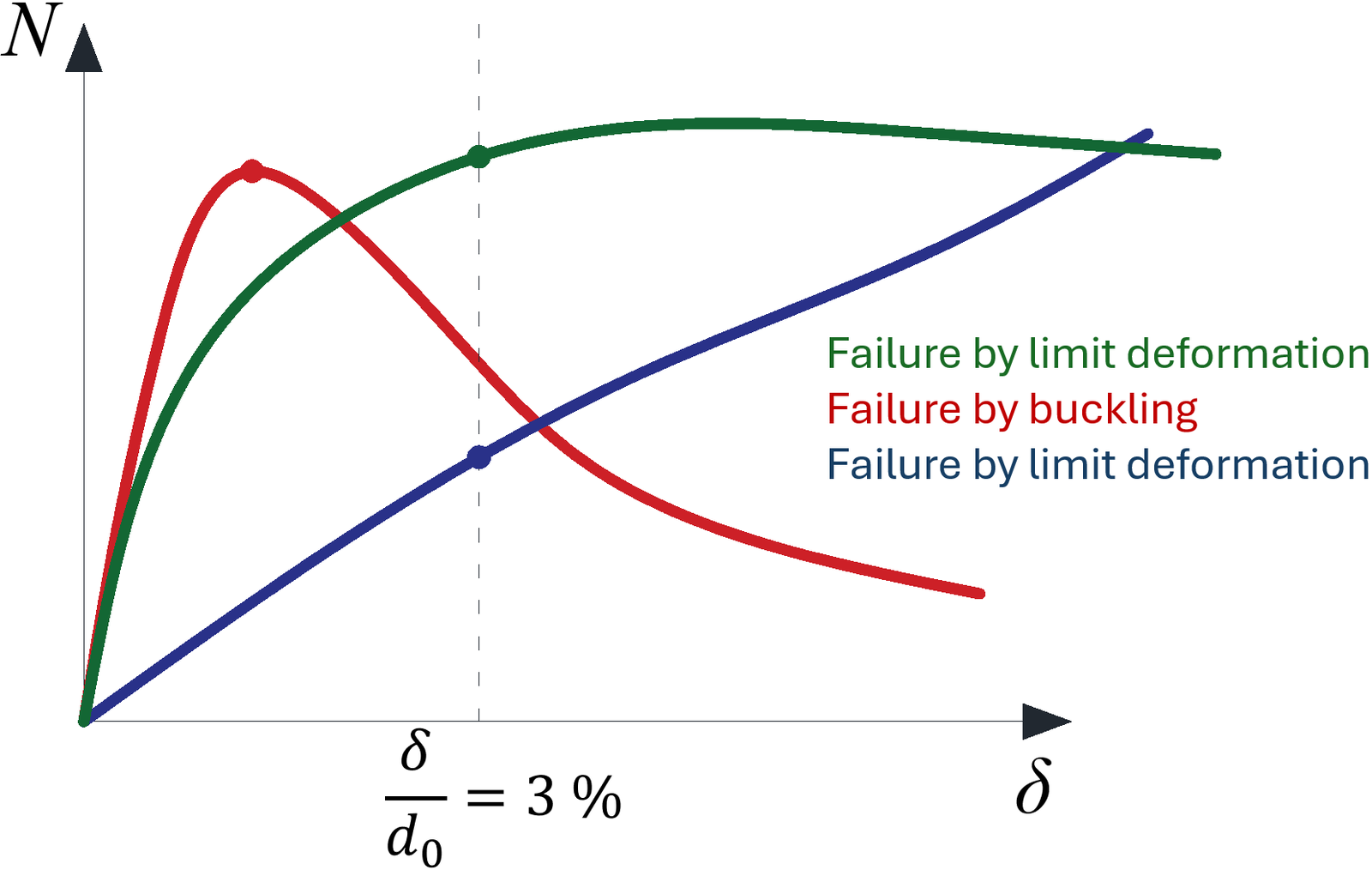
Typické diagramy zatížení-deformace pro přípoje dutých profilů; červená křivka je pro tenkostěnný prvek zatížený tlakem, zelená křivka pro běžné prvky zatížené tlakem, modrá křivka je např. pro X-přípoj zatížený tahem
Geometricky a materiálově nelineární analýza (GMNA)
V případě některých přípojů dutých profilů, zejména s vysokým poměrem průměru k tloušťce, nemusí geometricky lineární analýza zachytit chování přípoje s dostatečnou přesností a jeho únosnost může být podhodnocena nebo nadhodnocena. Doporučuje se použít pokročilejší geometricky a materiálově nelineární analýzu pro přípoje dutých profilů, i když je výpočetní čas mírně vyšší. Pokud je v Nastavení normy vybrána analýza GMNA pro duté profily, je GMNA použita místo geometricky lineární a materiálově nelineární analýzy (MNA, používané jako standard v IDEA Statica Connection) pro modely s prvkem z dutého profilu jako nosným prvkem.
Poznámka: Pokud nosný prvek není dutý profil, je řešič GMNA pro analýzu celého modelu přípoje deaktivován bez ohledu na nastavení v nastavení normy (GMNA zapnuto nebo vypnuto).
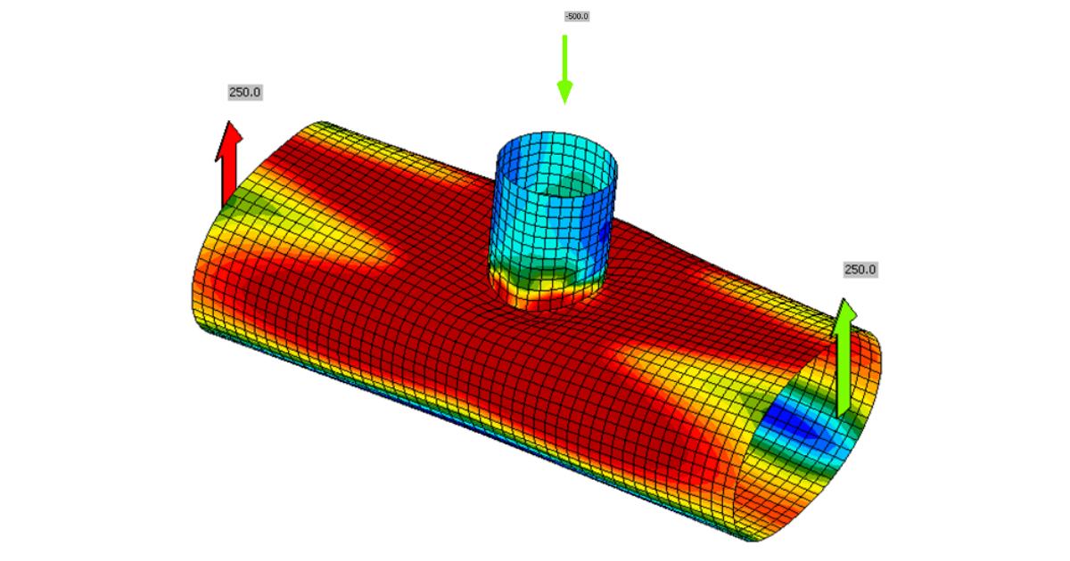
Deformace průřezu na konci modelu ze skořepinových prvků
Průřez se může deformovat na koncích modelu tvořeného skořepinovými prvky. Přípoje dutých profilů vyžadují relativně dlouhé prvky – až 10násobek průměru průřezu. Za částí modelu tvořenou skořepinovými prvky je umístěn kondenzovaný superprvek. To umožňuje rychlejší výpočet se stejnou přesností jako plný model tvořený skořepinovými prvky. Kondenzovaný superprvek má pouze elastické materiálové vlastnosti, což znamená, že plastická přetvoření způsobená zkoumaným způsobem porušení by neměla dosáhnout konce modelu ze skořepinových prvků. Z tohoto důvodu přesahuje skořepinový model ve výchozím nastavení o 1,25násobek výšky průřezu (upravitelné v Nastavení normy) za poslední výrobní operaci.
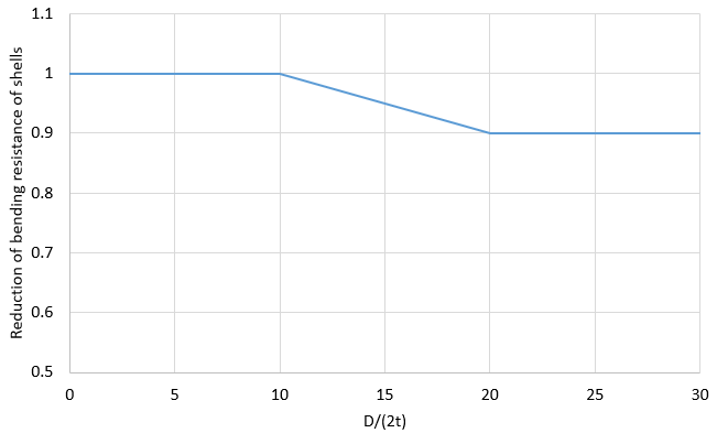
Ohybová únosnost skořepiny snížená pro duté profily (imperfekcí)
Únosnosti přípojů dutých profilů v normách jsou stanoveny metodou způsobů porušení, která využívá modely proložení křivkou určené z experimentů a pokročilých numerických modelů. Skutečná konstrukce obsahuje počáteční imperfekce a zbytkové napětí, které nejsou zachyceny skořepinovými modely v IDEA StatiCa Connection. Pro dosažení bližší shody s výsledky norem je vliv zbytkového napětí a počátečních imperfekcí simulován snížením ohybové únosnosti skořepin dutých profilů s vysokým poměrem D/(2t).
Typ analýzy únavy neposkytuje žádnou konečnou únosnost ani počet cyklů, které detail vydrží. Poskytuje pouze vstupy pro další výpočty podle norem.
Vždy musí být nastaveny alespoň dva zatěžovací stavy. První zatěžovací stav je referenční. Předpokládá se, že obsahuje například vlastní tíhu konstrukce a může obsahovat nulová zatížení. Ostatní zatěžovací stavy simulují únavová zatížení. Nominální normálové a smykové napětí poskytované IDEA StatiCa je rozsah napětí mezi únavovým zatížením, např. LE2, a referenčním zatěžovacím stavem.
Například smykové napětí v určitém místě je 50 MPa v referenčním zatěžovacím stavu a 180 MPa v LE2. Zobrazené nominální smykové napětí v tomto místě je:
Je třeba poznamenat, že v důsledku únavových zatížení by nemělo docházet k plastizaci plechů, jinak dochází ke zkreslení rozsahů napětí.
Napětí jsou k dispozici pro:
- Šrouby
- Svary
- Plechy
Šrouby
U šroubů se napětí stanoví jednoduše vydělením síly příslušnou plochou:
kde:
- – tahová síla ve šroubu
- – plocha průřezu šroubu v tahu
- – smyková síla ve šroubu; pokud existuje více střižných rovin, použije se nejvyšší smyková síla
- – plocha šroubu odolávající smyku; plocha průřezu v tahu, pokud závity protínají střižnou rovinu, jinak hrubý průřez
Svary
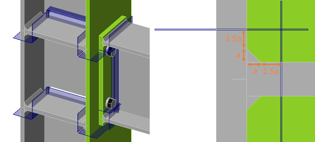
Svary v CBFEM se skládají z prvku svaru s víceuzlovými vazbami spojujícími plechy. Rozložení napětí ve svaru je narušeno vazbami, a proto se napětí odečítají z řezu umístěného ve vzdálenosti 1,5násobku velikosti nožičky od paty svaru. Pro oboustranný koutový svar jsou vytvořeny tři řezy. Dva řezy patří do stejné kategorie detailu a zobrazuje se pouze více namáhaný z nich. Zobrazuje se maximální normálové napětí a odpovídající smykové napětí ve stejném místě, jakož i maximální smykové napětí a odpovídající normálové napětí ve stejném místě.
Viz také vylepšení analýzy únavy ve verzi 22.0.
Plechy
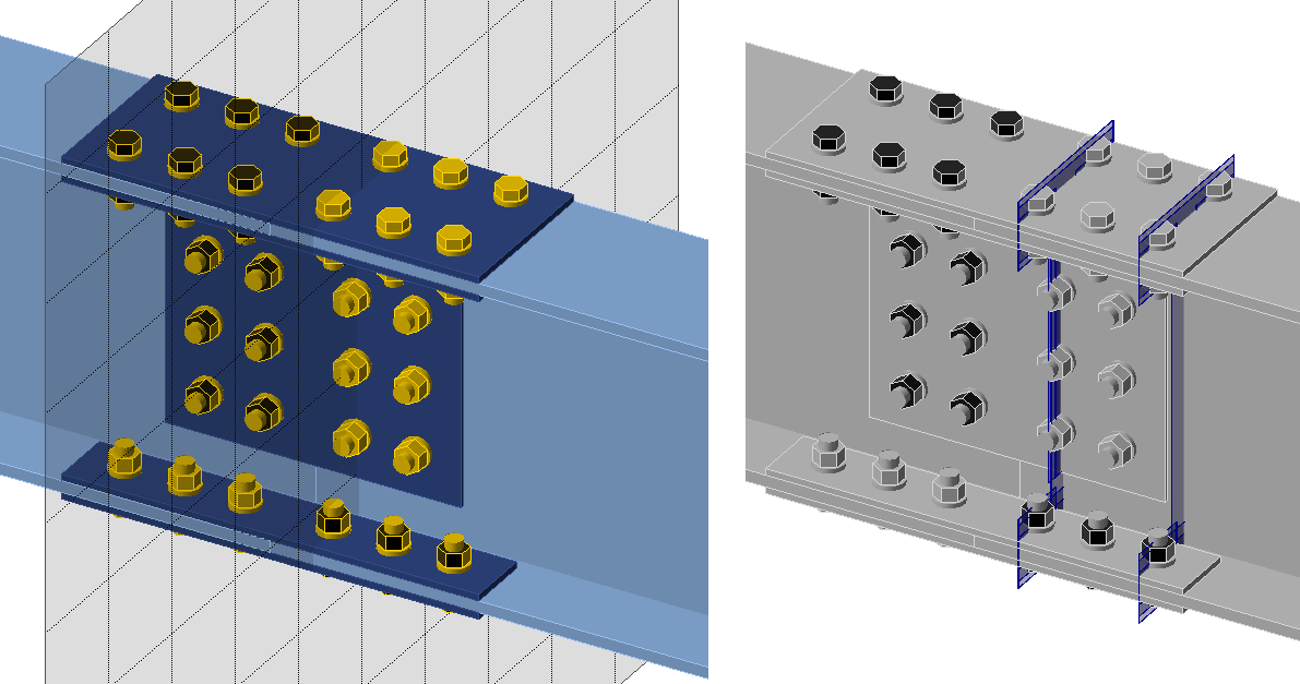
Napětí v pleších lze vizualizovat vytvořením uživatelsky definovaného řezu pomocí výrobní operace Pracovní rovina. Na obrázku níže byly vytvořeny dvě pracovní roviny pro zobrazení napětí v okolí otvorů pro šrouby. Zobrazuje se maximální normálové napětí a odpovídající smykové napětí ve stejném místě, jakož i maximální smykové napětí a odpovídající normálové napětí ve stejném místě.
Teplota
V IDEA StatiCa Member uživatel nastaví teplotu pro celý model. Všechny entity v modelu mají nastavenou teplotu.
V IDEA StatiCa Connection může uživatel nastavit teplotu pro každý dílec nebo plech zvlášť. Předpokládá se, že teplota spojovacích prvků - šroubů a svarů - je podle připojovaného plechu s nejvyšší teplotou.
Teplotu prvků a plechů ve spojích lze stanovit podle EN 1993-1-2, čl. 4.2.5 Vývoj teploty oceli a D.3 Teplota spojů při požáru.
Tepelné vlastnosti ocelových částí jsou stanoveny dle EN 1993-1-2:
- Měrné teplo – čl. 3.4.1.2
- Tepelná vodivost – čl. 3.4.1.3
Všimněte si, že teplotní roztažnost není v IDEA StatiCa použita, protože odpovídající vnitřní síly jsou závislé na okrajových podmínkách a musí být stanoveny na základě globální analýzy. Je doporučeno, aby do účinků zatížení byly síly od účinky teplotní roztažnosti dodatečně přidány.
Degradace materiálu
Degradace materiálu ocelových plechů je k dispozici podle tří norem:
- EN 1993-1-2 – tab. 3.1
- AISC 360-16 – tab. A-4.2.1
- CSA S16-14 – tab. K.1
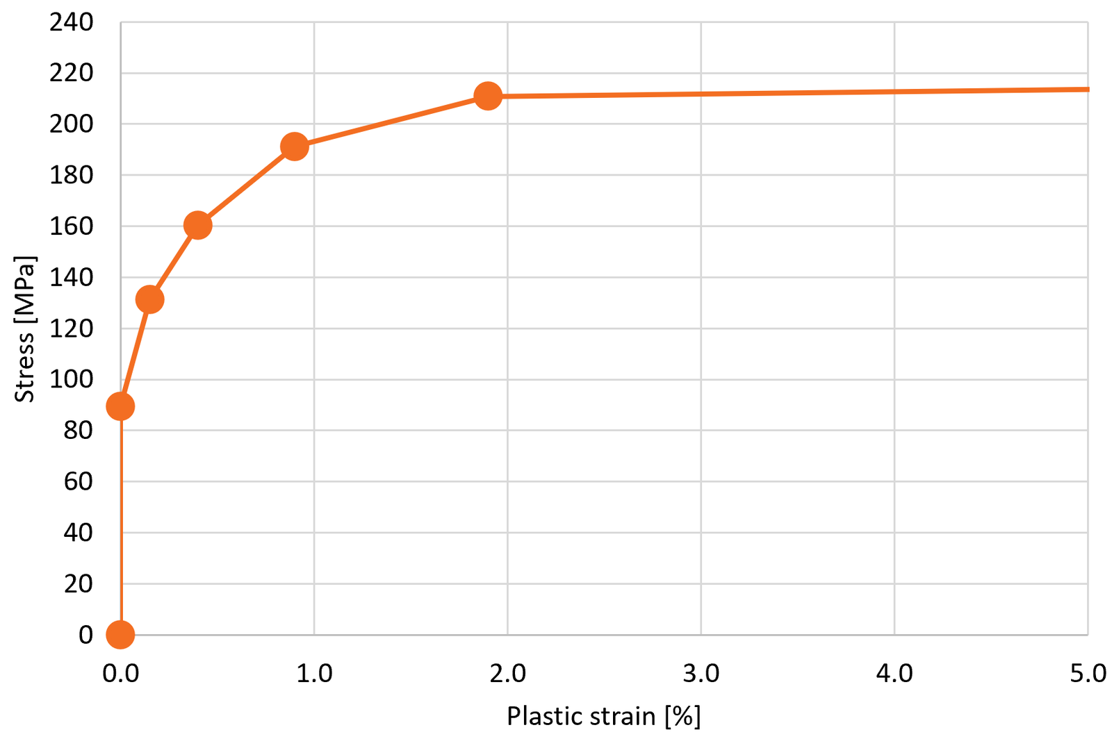
Multilineární materiálový diagram se používá pro ocelové plechy se šesti body podle EN 1993-1-2 – obr. 3.1. Příklad je uveden pro ocel třídy S355, degradaci materiálu podle EN 1993-1-2 – tabulka 3.1 a teplotu . Sklon plastické větve za mezí kluzu je . Redukční součinitele pro modul pružnosti , pro mez proporcionality a mez kluzu jsou 0,426, 0,252 a 0,594. Předpokládá se, že plastické přetvoření se od meze proporcionality zvyšuje.
| Kmen | Plastické namáhání | Stres | |
| [%] | [%] | [MPa] | |
| 0 | 0.00 | 0.00 | 0.0 |
| 1 | 0.10 | 0.00 | 89.5 |
| 2 | 0.25 | 0.15 | 131.4 |
| 3 | 0.50 | 0.40 | 160.5 |
| 4 | 1.00 | 0.90 | 191.3 |
| 5 | 2.00 | 1.90 | 210.9 |
| 6 | 15.00 | 14.90 | 222.5 |
Degradace materiálu šroubů je možná podle tří norem:
- EN 1993-1-2 – tabulka D.1
- AISC 360-16 – tabulka A-4.2.3
- CSA S16-14 – Tabulka K.3
Degradace materiálu svarů je k dispozici podle jedné normy:
- EN 1993-1-2 – tabulka D.1
Snižuje se pouze odolnost šroubů a svarů. Jejich tuhost zůstává stejná jako při okolní teplotě.
Tepelná roztažnost je zanedbávána a v žádném modelu se nepředpokládá. V případě potřeby by měly být účinky tepelné roztažnosti simulovány přidaným zatížením.
Posouzení
Ocelové plechy jsou standardně kontrolovány na plastické přetvoření 5 %.
V Eurokódu se pro posudky šroubů a svarů používá vyhrazený dílčí součinitel spolehlivosti pro posouzení požární odolnosti . Ve všech ostatních normách se používají standardní součinitele únosnosti nebo bezpečnosti. Deformační křivky a posudek šroubů a svarů jsou redukovány součiniteli a v závislosti na nastavené teplotě.
Předpokládá se, že předpjaté šrouby prokluzují, a kontrolují se jako běžné šrouby těsně utažené.
Teplota betonového bloku a kotev není známa a příslušné prvky nejsou v posouzení požáru posouzeny.
Tuhost
Analýza tuhosti není v současné době pro posouzení požáru k dispozici. Doporučuje se použít analýzu tuhosti pro okolní teplotu a vynásobit tuhost redukčním součinitelem pro modul pružnosti .
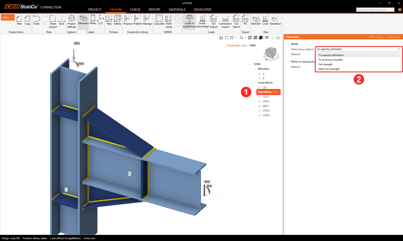
V IDEA StatiCa Connection jsou všem uživatelům k dispozici dvě strategie dimenzování svarů:
- na plnou únosnost
- s nadpevností
Pro uživatele Eurokódu jsou k dispozici dvě další:
- na odhadovanou kapacitu
- na minimální tažnost
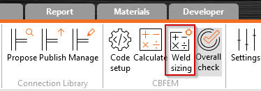
Metoda dimenzování svarů se zadává v dialogu Operace.
Při spuštění dimenzování svarů je každý koutový svar v modelu upraven podle zvolené metody dimenzování. Obecně platí, že velikost svarů se bude zvyšovat v tomto pořadí:
- Na odhadovanou kapacitu
- Na minimální tažnost
- Na plnou únosnost
- S nadpevností
Metody jsou podrobně popsány níže.
Na odhadovanou kapacitu
Dimenzování svarů na odhadovanou kapacitu automaticky poskytuje velikosti svarů, které jsou dostatečně únosné pro přenos zadaných zatížení.
Odhad kapacity svaru je prvním využitím strojového učení v IDEA StatiCa. V současné době je implementován pouze pro Eurokód. Únosnost svaru je stanovena podle nejvíce namáhaného prvku svaru. Využití svaru je proto vysoce nelineární. Únosnost celé délky je odhadována algoritmem strojového učení na základě rozložení napětí podél délky svaru.
Dimenzování svarů na odhadovanou kapacitu vyžaduje výsledky výpočtu. Velikost koutových svarů se upravuje podle následujícího vzorce:
kde:
- – upravená velikost koutového svaru
- – dříve nastavená velikost koutového svaru
- – odhad kapacity na základě algoritmu strojového učení zobrazený v posouzení svaru
- – cílové využití v Nastavení → Návrh → Automatický návrh → Dimenzování svarů
Výsledná hodnota je zaokrouhlena nahoru podle Předvolby → Jednotky aplikace → Zaokrouhlení nových entit → Velikost svaru.
Upozorňujeme, že velikosti svarů jsou omezeny konstrukčními zásadami, např. velikost svaru nesmí být menší než 3 mm (EN 1993-1-8 – 4.5.2). Tyto konstrukční zásady jsou dodržovány. Mějte také na paměti, že více svarů v IDEA StatiCa je často nastaveno jednou hodnotou. V těchto případech je velikost nastavena podle nejvíce využitého svaru.
K dispozici je také výpočetní smyčka. Pokud je metoda dimenzování svarů nastavena na odhadovanou kapacitu, provede se:
- Dimenzování koutových svarů na plnou únosnost
- Výpočet modelu
- Dimenzování koutových svarů na odhadovanou kapacitu
- Výpočet modelu
Svary jsou poté nastaveny na cílové využití nebo pod něj jediným kliknutím.
Na minimální tažnost
Dimenzování svarů na minimální tažnost automaticky zajišťuje svarové přípoje dostatečně únosné k zabránění křehkého porušení. Únosnost svaru umožňuje počáteční plastifikaci plechu, avšak v konečném důsledku dojde k přetržení svaru.
Požadavek na minimální tažnost svarových spojů je uveden v FprEN 1993-1-8:2023 – 6.9(4). Vychází z nizozemské národní přílohy EN 1993-1-8, kde je pevný poměr únosnosti svaru k únosnosti plechu 0,8. Je také zahrnut v hojně používaných Green books z Velké Británie, konkrétně v kapitolách C2 a C3. Pevný poměr je však vhodný pouze pro ocel třídy S355. V druhé generaci Eurokódu je tento požadavek rozšířen na všechny třídy oceli.
Tento požadavek je pro oboustranné koutové svary ověřován pomocí:
kde:
- – účinná výška koutového svaru
- – tloušťka plechu připojeného hranou
- – korelační součinitel svaru
- – součinitel spolehlivosti pro šrouby a svary; upravitelný v Nastavení normy
- – mez kluzu plechu
- – pevnost svaru v tahu
- – součinitel spolehlivosti pro plechy; upravitelný v Nastavení normy
Účinná výška jednostranného koutového svaru je dvakrát větší než u oboustranného koutového svaru.
Upozorňujeme, že metoda je vhodná pro příčně namáhané svary a funguje, pokud je plech připojen celou svou šířkou.
Na plnou únosnost
Dimenzování svarů na plnou únosnost automaticky zajišťuje svary, které jsou únosnější než připojený plech. Ve výpočtu se předpokládá, že plechy jsou namáhány tahem a svary příčně jako nejhorší případ z hlediska únosnosti a tažnosti svaru. Tento návrh je vhodný k zamezení křehkého porušení svarů při statickém zatížení.
Tento přístup je také zahrnut v hojně používaných Green books z Velké Británie, konkrétně v kapitole C1.
Tento požadavek je pro oboustranné koutové svary ověřován pomocí:
kde:
- – účinná výška koutového svaru
- – tloušťka plechu připojeného hranou
- – korelační součinitel svaru
- – součinitel spolehlivosti pro šrouby a svary; upravitelný v Nastavení normy
- – mez kluzu plechu
- – pevnost svaru v tahu
- – součinitel spolehlivosti pro plechy; upravitelný v Nastavení normy
Upozorňujeme, že metoda je vhodná pro příčně namáhané svary a funguje, pokud je plech připojen celou svou šířkou.
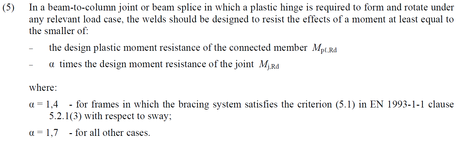
S nadpevností
Dimenzování svarů s nadpevností automaticky zajišťuje svary, které jsou výrazně únosnější než připojený plech. Součinitel nadpevnosti se zadává v Nastavení → Návrh → Automatický návrh → Dimenzování svarů. Výchozí hodnota 1,4 je převzata z EN 1993-1-8 – 6.2.3 (5) pro vytvoření plastického kloubu.
Ve výpočtu se předpokládá, že plechy jsou namáhány tahem a svary příčně jako nejhorší případ z hlediska únosnosti a tažnosti svaru. Tento návrh je vhodný k zamezení křehkého porušení svarů při plastickém návrhu nebo cyklickém zatížení. Upozorňujeme, že velká velikost svaru automaticky nezaručuje vysokou tažnost. Naopak může vést k nadměrným zbytkovým napětím a deformacím způsobeným smrštěním svaru.
Tento požadavek je pro oboustranné koutové svary ověřován pomocí:
kde:
- – účinná výška koutového svaru
- – tloušťka plechu připojeného hranou
- – korelační součinitel svaru
- – součinitel spolehlivosti pro šrouby a svary; upravitelný v Nastavení normy
- – mez kluzu plechu
- – pevnost svaru v tahu
- – součinitel spolehlivosti pro plechy; upravitelný v Nastavení normy
- – součinitel nadpevnosti zadaný v Nastavení → Návrh → Automatický návrh → Dimenzování svarů
Upozorňujeme, že metoda je vhodná pro příčně namáhané svary a funguje, pokud je plech připojen celou svou šířkou.