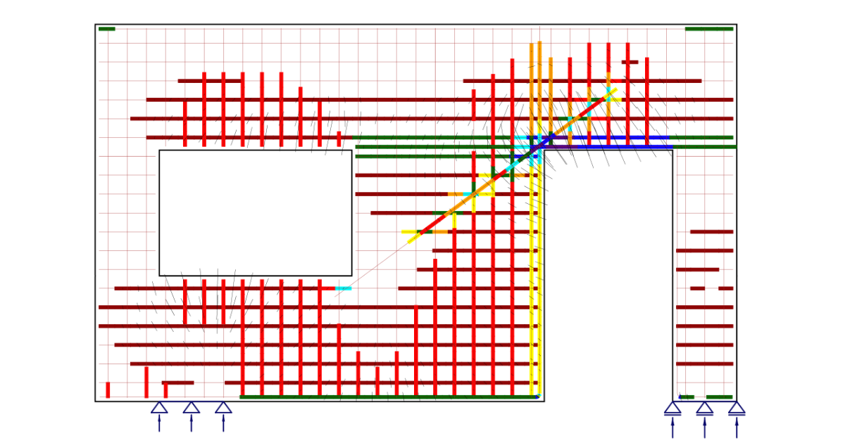
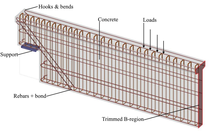
A betonszerkezeti elemek tervezése és ellenőrzése általában szelvény (1D-elem) vagy pont (2D-elem) szintjén történik. Ezt az eljárást minden szerkezettervezési szabvány leírja, pl. az EN 1992-1-1 vagy az ACI 318-19, és a mindennapi mérnöki gyakorlatban is ezt alkalmazzák. Azonban nem mindig ismert vagy tartják be, hogy ez az eljárás csak olyan területeken alkalmazható, ahol a sík alakváltozás-eloszlásra vonatkozó Bernoulli–Navier-hipotézis érvényes (ezeket B-régióknak nevezzük). Azokat a helyeket, ahol ez a hipotézis nem alkalmazható, diszkontinuitási vagy zavart régióknak (D-régióknak) nevezzük. Az 1D-elemek B- és D-régióira példák az (1. ábrán) láthatók. Ilyenek például a támaszkodási területek, a koncentrált terhelések alkalmazási helyei, a keresztmetszet hirtelen változásának helyei, nyílások stb. Betonszerkezetek tervezésekor számos egyéb D-régióval is találkozunk, mint például falak, hídfőtartók, konzolok stb.

\[ \textsf{\textit{\footnotesize{Fig. 1\qquad Discontinuity regions (Navrátil et al. 2017)}}}\]

A múltban a diszkontinuitási régiók méretezéséhez félempirikikus tervezési szabályokat alkalmaztak. Szerencsére ezeket a szabályokat az elmúlt évtizedekben nagyrészt felváltották a rácsmodellek (Schlaich et al., 1987) és a feszültségmezők (Marti 1985), amelyek megjelennek a jelenlegi tervezési szabványokban, és a tervezők ma is gyakran alkalmazzák őket. Ezek a modellek mechanikailag következetesek és hatékony eszközök. Megjegyzendő, hogy a feszültségmezők általában lehetnek folytonosak vagy nem folytonosak, és a rácsmodellek a nem folytonos feszültségmezők egy speciális esetét képezik.

A számítástechnikai eszközök elmúlt évtizedekben bekövetkezett fejlődése ellenére a Strut-and-Tie modellek lényegében még mindig kézi számításként kerülnek alkalmazásra. Valós szerkezeteknél való alkalmazásuk fáradságos és időigényes, mivel iterációk szükségesek, és több teherkombinációt kell figyelembe venni. Ezen túlmenően ez a módszer nem alkalmas a használhatósági kritériumok (alakváltozások, repedésszélességek stb.) ellenőrzésére.

A statikus mérnökök igénye egy megbízható és gyors eszköz iránt a D-régiók tervezéséhez vezetett a Compatible Stress Field Method kifejlesztésének döntéséhez, amely egy számítógéppel segített feszültségmező-tervezési módszer, amely lehetővé teszi a síkban terhelt szerkezeti betonszerkezeti elemek automatikus tervezését és ellenőrzését.

A Compatible Stress Field Method (CSFM) egy folytonos, végeselem-alapú feszültségmező-elemzési módszer, amelyben a klasszikus feszültségmező-megoldásokat kinematikai megfontolásokkal egészítik ki, azaz az alakváltozási állapotot a szerkezet egészén értékelik. Ennek megfelelően a beton hatékony nyomószilárdsága automatikusan számítható a keresztirányú alakváltozás állapota alapján, hasonlóan a nyomási lágyulást figyelembe vevő nyomásmező-elemzésekhez (Vecchio and Collins 1986; Kaufmann and Marti 1998) és az EPSF módszerhez (Fernández Ruiz and Muttoni 2007). Ezen túlmenően a CSFM figyelembe veszi a húzási merevítő hatást, reális merevséget biztosítva az elemeknek, és lefedi az összes tervezési szabvány előírást (beleértve a használhatósági és alakváltozási kapacitással kapcsolatos szempontokat is), amelyeket a korábbi megközelítések nem következetesen kezeltek. A CSFM a tervezési szabványok által megadott általános egytengelyű anyagmodelleket alkalmaz a betonra és a vasalásra. Ezek a tervezési szakaszban ismertek, ami lehetővé teszi a részleges biztonsági tényező módszer alkalmazását. Ezért a tervezőknek nem kell további, gyakran önkényes anyagtulajdonságokat megadniuk, amelyek általában a nemlineáris végeselem-elemzésekhez szükségesek, így a módszer tökéletesen alkalmas a mérnöki gyakorlatban való alkalmazásra.

A számítógéppel segített feszültségmezők statikus mérnökök általi alkalmazásának elősegítése érdekében ezeket a módszereket felhasználóbarát szoftverkörnyezetekben kell megvalósítani. Ennek érdekében a CSFM-et az IDEA StatiCa Detail-ben valósították meg; ez egy új, felhasználóbarát kereskedelmi szoftver, amelyet az ETH Zürich és az IDEA StatiCa szoftverszállító közösen fejlesztett ki a DR-Design Eurostars-10571 projekt keretében.

1.2 A CSFM főbb feltételezései és korlátai 2D-ben

A CSFM a beton maximális főnyomófeszültségét (σ_c₂_r) és a vasalás feszültségeit (σ_sr) a repedéseknél veszi figyelembe, miközben elhanyagolja a beton húzószilárdságát (σ_c₁_r = 0), kivéve annak a vasalásra gyakorolt merevítő hatását. A húzási merevítő hatás figyelembevétele lehetővé teszi a vasalás átlagos alakváltozásainak (ε_m) szimulálását. Fiktív, forgó, feszültségmentes repedéseket vesznek figyelembe, amelyek csúszás nélkül nyílnak (2a. ábra), és a repedéseknél fennálló egyensúlyt a vasalás átlagos alakváltozásaival együtt szintén figyelembe veszik.

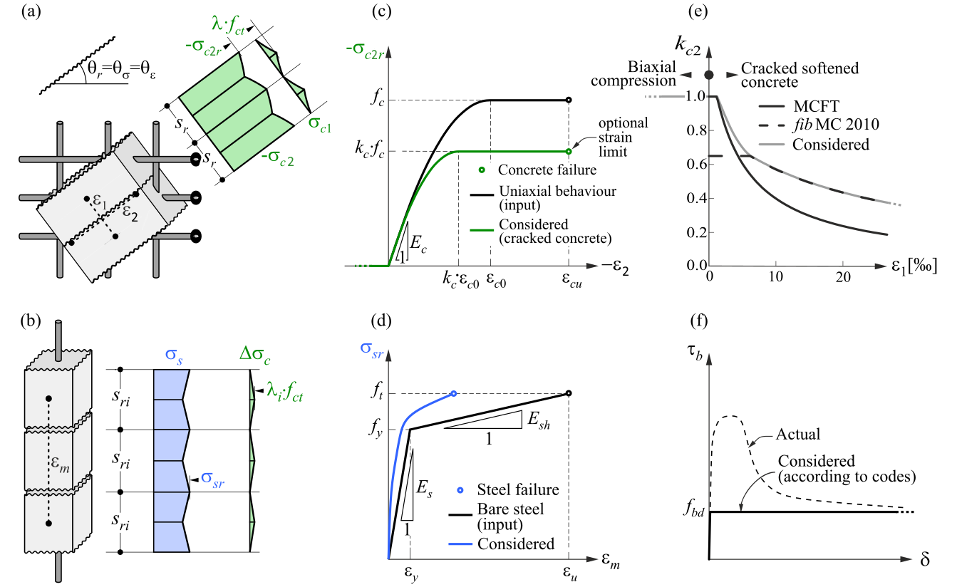
\( \textsf{\textit{\footnotesize{Fig. 2\qquad Basic assumptions of the CSFM: (a) principal stresses in concrete; (b) stresses in the reinforcement direction;}}}\) \( \textsf{\textit{\footnotesize{(c) stress-strain diagram of concrete in terms of maximum stresses with consideration of compression softening;}}}\) \( \textsf{\textit{\footnotesize{(d) stress-strain diagram of reinforcement in terms of stresses at cracks and average strains; (e) compression softening}}}\) \( \textsf{\textit{\footnotesize{law; (f) bond shear stress-slip relationship for anchorage length verifications.}}}\)

Egyszerűségük ellenére hasonló feltételezések bizonyítottan pontos előrejelzéseket adnak síkbeli terhelésnek kitett vasalt szerkezeti elemeknél (Kaufmann 1998; Kaufmann és Marti 1998), feltéve, hogy a biztosított vasalás elkerüli a repedéskor bekövetkező rideg tönkremenetelt. Továbbá a beton húzószilárdságának a végső teherbíráshoz való hozzájárulásának figyelmen kívül hagyása összhangban van a modern tervezési szabványok elveivel, amelyek többnyire a képlékenységi elméleten alapulnak.

Ugyanakkor a CSFM nem alkalmas karcsú elemekre harántirányú vasalás nélkül, mivel az ilyen elemek szempontjából meghatározó mechanizmusokat – mint az aggregátum-összekapaszkodás, a repedéscsúcsnál fennmaradó húzófeszültségek és a csaphatás – amelyek mindegyike közvetlenül vagy közvetve a beton húzószilárdságára támaszkodik, figyelmen kívül hagyja. Bár egyes tervezési szabványok lehetővé teszik az ilyen elemek méretezését félempirikus előírások alapján, a CSFM nem erre a potenciálisan rideg szerkezettípusra készült.

Beton

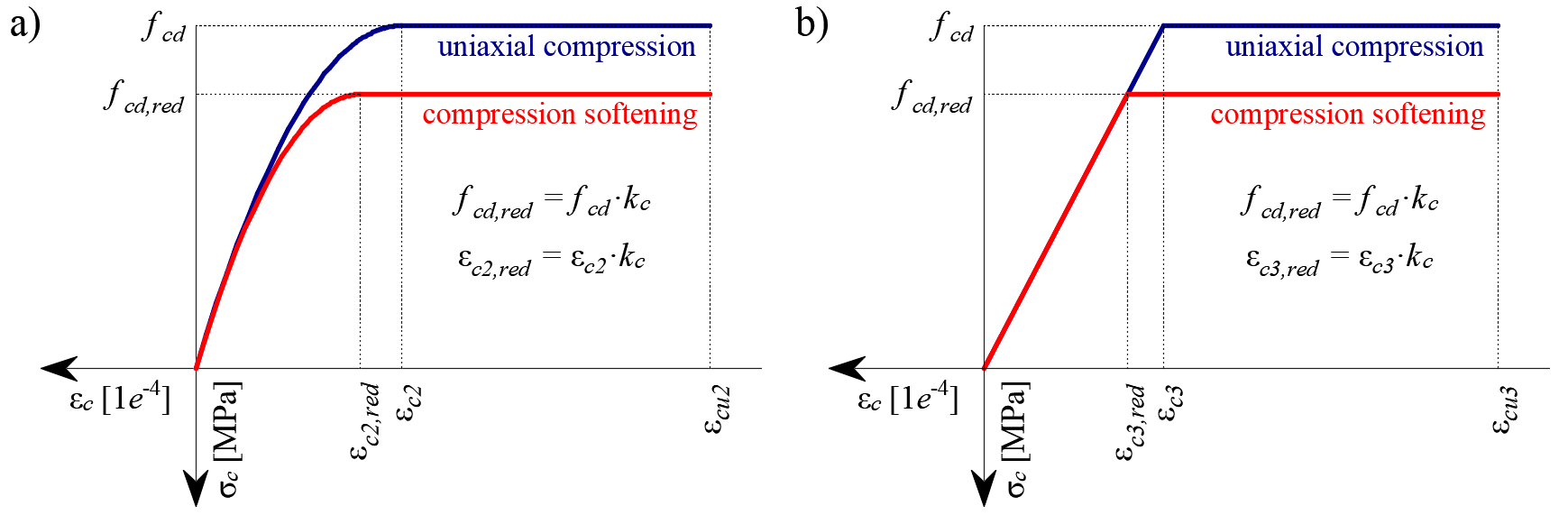
A CSFM-ben alkalmazott betonmodell a tervezési szabványok által a keresztmetszet-méretezéshez előírt egytengelyű nyomási alkotótörvényeken alapul, amelyek kizárólag a nyomószilárdsától függnek. A CSFM-ben alapértelmezés szerint a parabola-téglalap diagram (2c. ábra) kerül alkalmazásra, de a tervezők egyszerűsített rugalmas–ideálisan képlékeny összefüggést is választhatnak. Az ACI szabvány szerinti ellenőrzésnél kizárólag a parabola-téglalap feszültség-alakváltozás diagram használható. Amint korábban említettük, a húzószilárdságot elhanyagolják, ahogyan az a klasszikus vasbeton-tervezésben is szokásos.

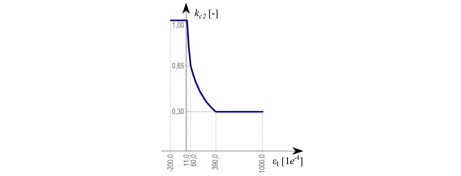
A repedezett betonra vonatkozó hatékony nyomószilárdságot automatikusan értékelik a főhúzó alakváltozás (ε₁) alapján a k_c₂ redukciós tényező segítségével, ahogyan azt a 2c. és 2e. ábra mutatja. Az alkalmazott redukciós összefüggés (2e. ábra) a fib Model Code 2010 nyírási ellenőrzésekre vonatkozó javaslatának általánosítása, amely 0,65-ös határértéket tartalmaz a hatékony betonszilárdság és a beton nyomószilárdsága maximális arányára vonatkozóan, ami más teherbírási esetekre nem alkalmazható.

Az IDEA StatiCa Detail CSFM-je nem alkalmaz explicit tönkremeneteli kritériumot a nyomott beton alakváltozásaira vonatkozóan (azaz a csúcsfeszültség elérése után végtelen képlékeny ágat feltételez). Ez az egyszerűsítés nem teszi lehetővé a nyomásban tönkremenő szerkezetek alakváltozási kapacitásának ellenőrzését. Ugyanakkor a végső teherbírásuk megfelelően becsülhető, ha a repedezett beton tényezőjén (k_c₂) túl (2e. ábra), a beton ridegségének szilárdság növekedésével arányos növekedését is figyelembe veszik a fib Model Code 2010-ben az alábbiak szerint definiált \( \eta_{fc} \) redukciós tényező segítségével:

\[f_{c,red} = k_c \cdot f_{c} = \eta _{fc} \cdot k_{c2} \cdot f_{c}\]

\[{\eta _{fc}} = {\left( {\frac{{30}}{{{f_{c}}}}} \right)^{\frac{1}{3}}} \le 1\]

ahol:

k_ca nyomószilárdság globális redukciós tényezője

k_c₂ a harántirányú repedések jelenlétéből adódó redukciós tényező

f_c a beton hengeres karakterisztikus szilárdsága (MPa-ban az \( \eta_{fc} \) definíciójához).

A számítás stabilitása miatt a k_c₂ tényező szintén csökkentésre kerül. Ez a csökkentés nem befolyásolja a szerkezeti elemek teljes teherbírását. Az f_cd értéket a beton terhelt szilárdságaként (méretezési érték) feltételezve, a k_c₂ értéke az alábbi szabályok szerint csökken.

σ_c₂_r < 0.11f_cd                                           k_c₂=1.0
0.11f_cd < σ_c₂_r < 0.37f_cd                          k_c₂ lineáris interpoláció 1,0 és a 2f. ábrán látható
                                                              grafikonból vett érték között
σ_c₂_r > 0.37f_cd                                           k_c₂ közvetlenül a 2f. ábra grafikonjából kerül leolvasásra

Vasalás

A tervezési szabványok által jellemzően meghatározott idealizált bilineáris feszültség-alakváltozás diagramot alkalmazzák a szabad vasalórudakra (2d. ábra). E diagram meghatározásához csupán a vasalás alapvető tulajdonságainak ismerete szükséges a tervezési fázisban (szilárdság és képlékenységi osztály). Felhasználó által definiált feszültség-alakváltozás összefüggés szintén megadható.

A húzási merevítő hatást a szabad vasalórúd bemeneti feszültség-alakváltozás összefüggésének módosításával veszik figyelembe, hogy visszaadják a betonba ágyazott rudak átlagos merevségét (ε_m).

Tapadási modell

A vasalás és a beton közötti tapadási csúszást a végeselem-modellben a 2f. ábrán bemutatott egyszerűsített merev–tökéletesen képlékeny alkotótörvény figyelembevételével modellezik, ahol f_bd a tervezési szabvány által az adott tapadási feltételekre meghatározott végső tapadási feszültség méretezési értéke (terhelt értéke).

Ez egy egyszerűsített modell, amelynek egyetlen célja a tapadási előírások ellenőrzése a tervezési szabványok szerint (azaz a vasalás lehorgonyzása). A lehorgonyzási hossz csökkentése horgok, hurkok és hasonló rúdalakzatok alkalmazásakor figyelembe vehető a vasalás végén meghatározott kapacitás megadásával, ahogyan azt a továbbiakban ismertetjük.

1.3 Vasalástervezési eszközök

Munkafolyamat és célok

A vasalástervezési eszközök célja a CSFM-ben, hogy segítsék a tervezőket a vasalási rudak helyének és szükséges mennyiségének hatékony meghatározásában. A következő eszközök állnak rendelkezésre a felhasználó segítésére / irányítására ebben a folyamatban: lineáris számítás és topológiai optimalizálás.

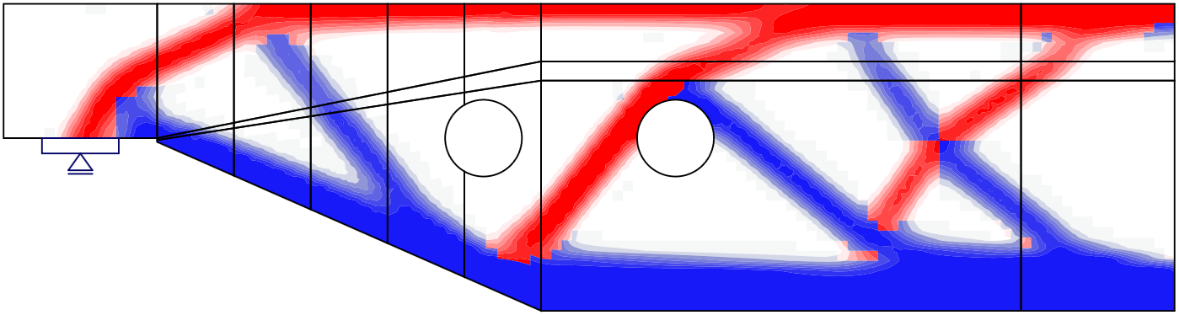
A vasalástervezési eszközök egyszerűsítettebb anyagmodelleket alkalmaznak, mint a szerkezet végső ellenőrzéséhez használt modellek. Ezért az ebben a lépésben meghatározott vasalást előtervezésnek kell tekinteni, amelyet a végső ellenőrzési lépés során meg kell erősíteni/finomítani. A különböző vasalástervezési eszközök alkalmazását a 3. ábrán látható modellen mutatjuk be, amely egy egyszerűen alátámasztott, változó magasságú gerenda egyik végét ábrázolja, amelyre egyenletesen elosztott terhelés hat.

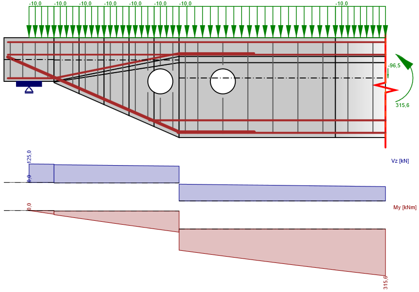
\[ \textsf{\textit{\footnotesize{Fig. 3\qquad Model used to illustrate the use of the reinforcement design tools.}}}\]

Lineáris analízis

A lineáris analízis lineárisan rugalmas anyagtulajdonságokat vesz figyelembe, és elhanyagolja a vasalást a betonrégióban. Ezért egy nagyon gyors számítás, amely első betekintést nyújt a húzott és nyomott területek elhelyezkedésébe. Ilyen számítás eredményét mutatja a 4. ábra.

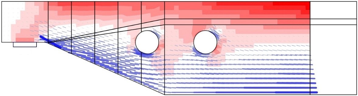
\[ \textsf{\textit{\footnotesize{Fig. 4\qquad Results from the linear analysis tool for defining reinforcement layout}}}\]

\[ \textsf{\textit{\footnotesize{(red: areas in compression, blue: areas in tension).}}}\]

Topológiai optimalizálás

A topológiai optimalizálás egy olyan módszer, amelynek célja az anyag optimális eloszlásának meghatározása egy adott térfogatban, egy bizonyos terhelési konfiguráció esetén. Az Idea StatiCa Detail-ben implementált topológiai optimalizálás lineáris végeselem-modellt alkalmaz. Minden végeselem relatív sűrűsége 0-tól 100%-ig terjedhet, amely a felhasznált anyag relatív mennyiségét jelöli. Ezek az elemek sűrűségei az optimalizálási feladat paraméterei. Az eredményül kapott anyageloszlás akkor tekinthető optimálisnak az adott terhelési készletre, ha minimalizálja a rendszer teljes alakváltozási energiáját. Definíció szerint az optimális eloszlás egyben az a geometria is, amely a legnagyobb lehetséges merevséggel rendelkezik az adott terhelésekre.

Az iteratív optimalizálási folyamat homogén sűrűségeloszlással kezdődik. A számítás több teljes térfogathányad esetén kerül elvégzésre (20%, 40%, 60% és 80%), ami lehetővé teszi a felhasználó számára a legpraktikusabb eredmény kiválasztását. Az eredményül kapott alak rácsszerkezetekből áll nyomott rudakkal és húzott elemekkel, és az adott teherkombinációkra optimális alakot képviseli (5. ábra).

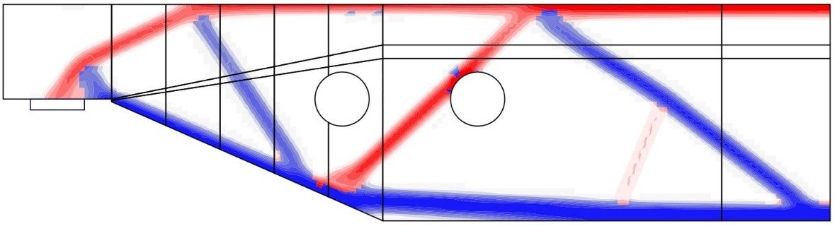
\[ \textsf{\textit{\footnotesize{Fig. 5\qquad Results from the topology optimization design tool with 20\% and 40\% effective volume}}}\]

\[ \textsf{\textit{\footnotesize{(red: areas in compression, blue: areas in tension).}}}\]

2 Az IDEA StatiCa Detail elemzési modellje

2.1 Bevezetés a végeselem-módszer implementációjába

A CSFM folytonos feszültségi tereket vesz figyelembe a betonban (2D végeselemek), amelyeket a vasalást reprezentáló diszkrét „rúd" elemek (1D végeselemek) egészítenek ki. Ezért a vasalás nem diffúzan van beágyazva a beton 2D végeselemekbe, hanem explicit módon modellezve és azokhoz kapcsolva. A számítási modellben síkfeszültségi állapotot feltételezünk.

\[ \textsf{\textit{\footnotesize{Fig. 6\qquad Visualization of the calculation model of a structural element (trimmed beam) in Idea StatiCa Detail.}}}\]

Modellezhető mind teljes falak és gerendák, mind pedig gerendák részletei (részei) (izolált diszkontinuitási régió, más néven csonkított vég). Falak és teljes gerendák esetén a megtámasztásokat úgy kell meghatározni, hogy (külsőleg) izostatikus (statikailag határozott) vagy hiperstatikus (statikailag határozatlan) szerkezet jöjjön létre. A gerendák csonkított végeinél a teherátadás egy speciális Saint-Venant átadási zóna segítségével valósul meg, amely biztosítja a feszültségek reális eloszlását az elemzett részlet-régióban.

2.2 Támaszok és terheléstovábbító elemek

Az építési folyamat során előforduló legtöbb helyzet modellezéséhez a CSFM-ben számos típusú támasz (7. ábra) és terheléstovábbító elem (8. ábra) áll rendelkezésre.

Támaszok

A ponttámasz többféleképpen modellezhető annak érdekében, hogy a feszültségek ne egy pontban koncentrálódjanak, hanem nagyobb területen oszoljanak el. Az első lehetőség az elosztott ponttámasz (7a. ábra), amely a szerkezeti elem szélén a terhelést egyenletesen osztja el a megadott szélességen.

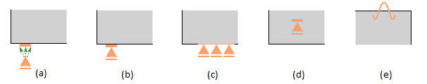
\[ \textsf{\textit{\footnotesize{Fig. 7\qquad Various types of supports:}}}\]

\[ \textsf{\textit{\footnotesize{(a) point distributed; (b) bearing plate; (c) line support; (d) patch support; (e) hanging.}}}\]

A patch support (7d. ábra) ezzel szemben csak egy meghatározott hatékony sugarú betonvolumenen belül helyezhető el. Merev elemekkel kapcsolódik a vasalási háló csomópontjaihoz ezen a sugáron belül. Ezért a patch support körül vasalási kalitkát kell meghatározni.

Egyes valós helyzetek pontosabb modellezéséhez a ponttámasznak két további változata áll rendelkezésre. Az első a meghatározott szélességű és vastagságú alátétlemezzel ellátott ponttámasz (7b. ábra). Az alátétlemez anyaga megadható, és az egész alátétlemez önállóan kerül hálózásra. A második lehetőség a függesztett támasz (7e. ábra), amely emelési horgonyok vagy emelési csapok modellezésére használható.

A vonalmenti támasz (7c. ábra) meghatározható egy élen (hosszának megadásával) vagy egy elemen belül (töröttvonal segítségével). Lehetőség van a merevség és/vagy a nemlineáris viselkedés megadására is (nyomásban/húzásban vagy csak nyomásban működő támasz).

Részletes leírás itt olvasható: Types of supports in IDEA StatiCa Detail

Terheléstovábbító elemek

A terhek szerkezetbe való bevezetése szintén többféleképpen modellezhető. Pontterhek esetén alátétlemez (8a. ábra) alkalmazható, hasonlóan a ponttámaszhoz, amely a koncentrált terhelést nagyobb területre osztja el egy meghatározott szélességű és vastagságú acéllemez segítségével.

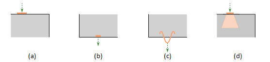
\[ \textsf{\textit{\footnotesize{Fig. 8\qquad Various types of load transfer components:}}}\]

\[ \textsf{\textit{\footnotesize{(a) bearing plate; (b) patch load; (c) hanging; (d) partially loaded area.}}}\]

A pontterhelés alkalmazható közvetlenül a szerkezet felületére meghatározott hatássugarral (a terhelés a beton elemekre hat), vagy egy patch load nevű speciális terheléstovábbító eszközön keresztül (8b. és 9. ábra). A patch load lehetővé teszi a terhelés közvetlen átadását a hatékony sugáron belül elhelyezkedő meghatározott vasalásra. A patch load helyes működéséhez meg kell határozni azokat a betonacél rudakat, amelyek a terheléssel össze lesznek kapcsolva (a vasalás tulajdonságaiban). Ha az összekapcsolt vasalás nincs meghatározva, a terheléstovábbítás mechanizmusa megegyezik a szerkezeti elem felületére helyezett pontterheléssel, és a terhelés a kényszerfeltételeken keresztül a beton elemekre, nem közvetlenül a vasalásra adódik át.

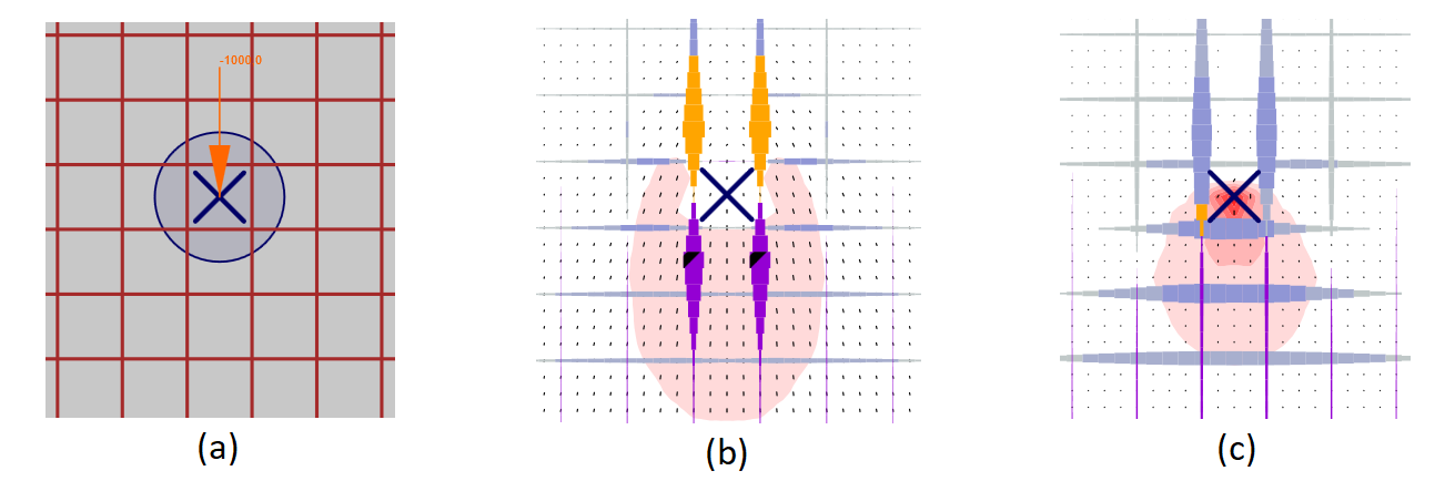
\[ \textsf{\textit{\footnotesize{Fig. 9\qquad Patch load: (a) load application; (b) load transferred through rebars (a group of bars for the load transfer is defined);}}}\]

\[ \textsf{\textit{\footnotesize{(c) load transferred through concrete (a group of bars for the load transfer is not defined).}}}\]

Az emelési horgonyok vagy emelési csapok függesztett terheléssel modellezhetők (8c. ábra). A felhasználó részlegesen terhelt területet is alkalmazhat (8d. ábra), amely lehetővé teszi a beton nyomási teherbírásának növelését az Eurocode szerint (ez a terheléstovábbító elem típus ACI szabvány alkalmazása esetén nem használható). A szerkezet vonalmenti terhelésekkel is terhelhető az éleken, általános töröttvonal mentén, vagy felületi terhelésekkel. A Detail alkalmazás képes az önsúlyt automatikusan figyelembe venni az analízis során.

2.3 Terhelésátadás gerendák levágott végeinél

Sok esetben egy szerkezeti elem csak egy részletét (részét) kell modelleznünk, például gerenda támaszt, a gerenda közepén lévő nyílást stb. Ez a megközelítés olyan támaszrendszerekhez vezethet, amelyek instabilak, de megengedhetők az IDEA StatiCa Detail-ben (beleértve a támasz nélküli esetet is). Ilyen esetekben azonban szükséges a szomszédos B-régióhoz való kapcsolódást képviselő keresztmetszetet is modellezni, beleértve az egyensúlyt kielégítő belső erőket is ebben a keresztmetszetben. Bizonyos esetekben (pl. gerenda támasz modellezésekor) ezeket a belső erőket a program automatikusan meg tudja határozni.

A B-régió és az elemzett diszkontinuitási régió között egy Saint-Venant átmeneti zóna jön létre automatikusan, hogy biztosítsa a reális feszültségeloszlást az elemzett régióban. Az átmeneti zóna szélessége a keresztmetszet magasságának felével egyenlő. Mivel a Saint-Venant zóna egyetlen célja a megfelelő feszültségeloszlás elérése a modell többi részében, ebből a területből nem jelennek meg eredmények az ellenőrzésben, és itt nem kerülnek figyelembevételre leállási kritériumok sem.

A Saint-Venant zóna azon éle, amely a gerenda levágott végét képviseli, merevként van modellezve, azaz elfordulhat, de síkban kell maradnia. Ez úgy valósul meg, hogy az él összes végeselem-csomópontját egy merev test elemmel (RBE2) a keresztmetszet tehetetlenségi középpontjában lévő külön csomóponthoz kapcsolják. Az elem belső erői ezután alkalmazhatók erre a csomópontra, ahogy a 10. ábrán látható.

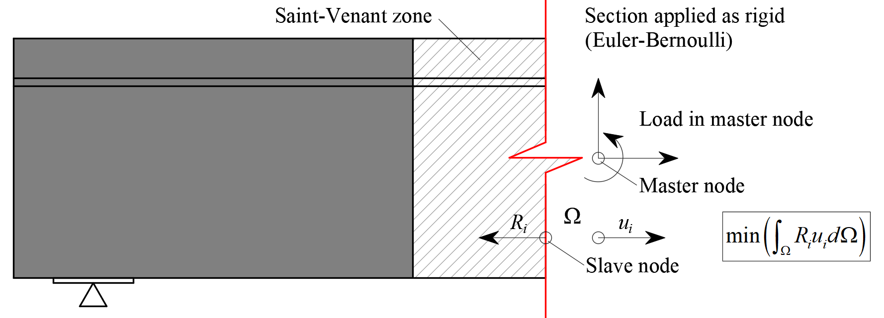
\[ \textsf{\textit{\footnotesize{Fig. 10\qquad Transfer of internal forces at a trimmed end.}}}\]

2.4 Keresztmetszetek geometriai módosítása

A keresztmetszet csökkentése automatikusan elvégzésre kerül a gerendaként vagy keretcsomópontként definiált szerkezeteknél (x-tengellyel és keresztmetszettel meghatározva). Ez a módosítás automatikusan alkalmazásra kerül a nagyon széles övekkel rendelkező keresztmetszeteken (11. ábra), és azon a feltételezésen alapul, hogy a nyomott rúd 45°-os szögben terjed ki a falból, így az említett csökkentett szélesség a terhelések átadására képes maximális szélesség.

Megjegyzendő, hogy a CSFM-ben alkalmazott hatékony övszélesség meghatározásának módszere eltér az EN 1992-1-1 (2015) 5.3.2.1 pontjában vagy az ACI 318-19 9.2.4.4 pontjában megadottól. A geometrián túl az Eurocode-alapú hatékony övszélességet explicit módon befolyásolják a szerkezet fesztávolságai és peremfeltételei.

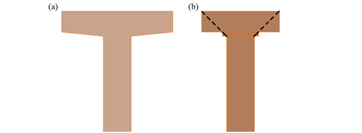
\[ \textsf{\textit{\footnotesize{Fig. 11\qquad Width reduction of a cross-section: (a) user input; (b) FE model – automatically determined reduced flange width.}}}\]

Vízszintes síkban elhelyezkedő vállak esetén (12. ábra) minden egyes váll öt szakaszra van osztva a hossza mentén. Ezeket a szakaszokat ezután állandó vastagságú falként modellezik, amely egyenlő a valódi vastagsággal az adott szakasz közepén.

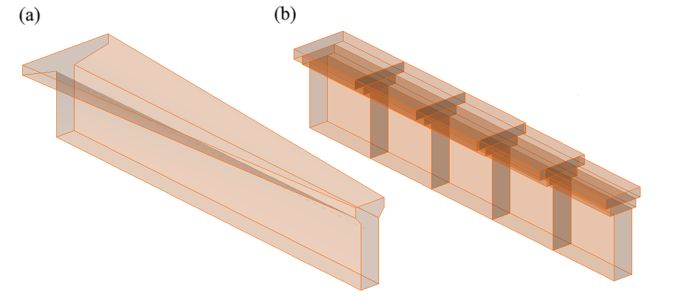
\[ \textsf{\textit{\footnotesize{Fig. 12\qquad Horizontal haunch: (a) user input; (b) FE model – a haunch automatically divided into five sections.}}}\]

2.5 Végeselem-típusok

A nemlineáris (inelasztikus) végeselem-analízis modellje több végeselem-típusból áll, amelyek a betont, a vasalást és a köztük lévő tapadást modellezik. A beton- és vasaláselemeket először egymástól függetlenül hálózzák be, majd többpontos kényszerfeltételek (MPC elemek) segítségével kapcsolják össze egymással. Ez lehetővé teszi, hogy a vasalás tetszőleges, relatív helyzetben legyen a betonhoz képest. Ha a lehorgonyzási hossz ellenőrzését is el kell végezni, tapadási és lehorgonyzási végponti rugóelemeket illesztenek be a vasalás és az MPC elemek közé.

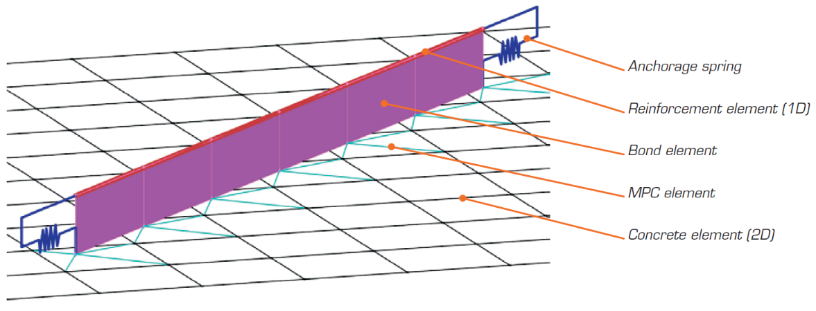
\[ \textsf{\textit{\footnotesize{Fig. 13\qquad Finite element model: reinforcement elements mapped to concrete mesh using MPC elements and bond elements.}}}\]

Beton

A betont négyszögletű és háromszögletű héjelemekkel modellezik: CQUAD4 és CTRIA3. Ezek négy, illetve három csomóponttal definiálhatók. Ezekben az elemekben kizárólag síkfeszültségi állapotot feltételeznek, azaz a z-irányú feszültségeket és alakváltozásokat nem veszik figyelembe.

Minden elemnek négy vagy három integrációs pontja van, amelyek az elem méretének körülbelül 1/4-énél helyezkednek el. Minden elem minden integrációs pontjában kiszámítják a főalakváltozások irányait: α₁, α₂. Mindkét irányban a főfeszültségeket σ_c₁, σ_c₂ és a merevségeket E₁, E₂ a megadott beton feszültség-alakváltozás diagram alapján értékelik ki, a 2. ábra szerint. Megjegyzendő, hogy a nyomási lágyulás hatása összekapcsolja a fő nyomási irány viselkedését a másik főirány tényleges állapotával.

Vasalás

A betonacél rudakat kétcsomópontos, 1D „rúd" elemekkel (CROD) modellezik, amelyek csak axiális merevséggel rendelkeznek. Ezeket az elemeket speciális „tapadási" elemekhez kapcsolják, amelyeket a betonacél rúd és a körülvevő beton közötti csúszási viselkedés modellezésére fejlesztettek ki. Ezeket a tapadási elemeket ezt követően MPC (többpontos kényszerfeltétel) elemek segítségével kapcsolják a betont reprezentáló hálóhoz. Ez a megközelítés lehetővé teszi a vasalás és a beton egymástól független hálózását, miközben összekapcsolásuk később biztosított.

Tapadási elemek

A lehorgonyzási hosszt a beton elemek (2D) és a betonacél rúd elemek (1D) közötti tapadási nyírófeszültségek végeselem-modellbe való beépítésével ellenőrzik. Ennek érdekében egy „tapadási" végeselem-típust fejlesztettek ki.

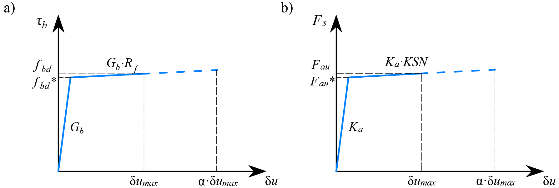
A tapadási elem definíciója hasonló a héjelemhez (CQUAD4). Szintén 4 csomóponttal definiált, de a héjjal ellentétben csak a két felső és két alsó csomópont közötti nyírásban rendelkezik nullától eltérő merevsége. A modellben a felső csomópontok a vasalást reprezentáló elemekhez, az alsó csomópontok a betont reprezentáló elemekhez kapcsolódnak. Ennek az elemnek a viselkedését a tapadási feszültség, τ_b, írja le, mint a felső és alsó csomópontok közötti csúszás, δ_u, bilineáris függvénye, lásd 14. ábra.

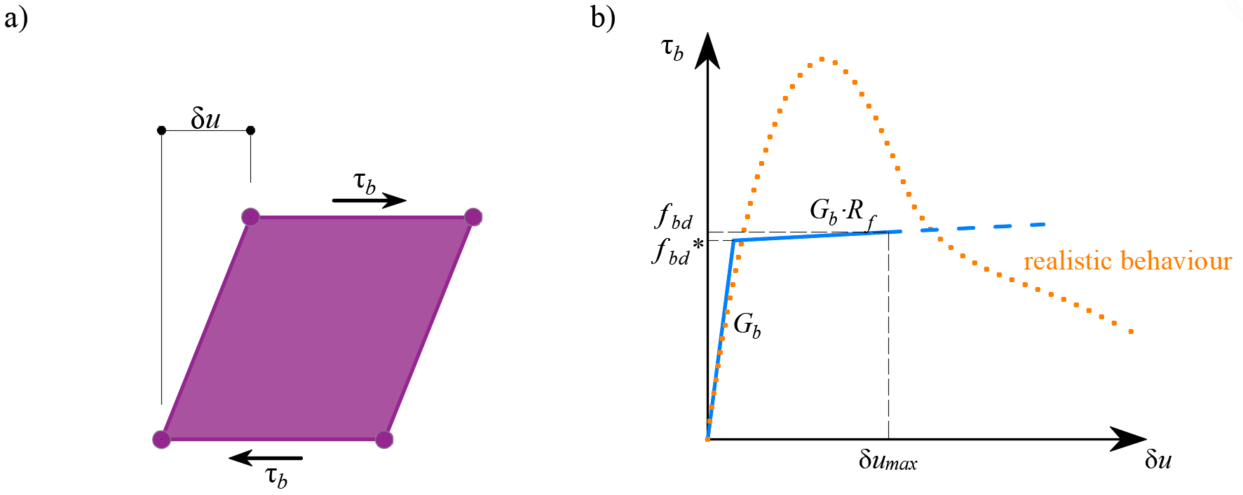
\[ \textsf{\textit{\footnotesize{Fig. 14\qquad (a) conceptual illustration of the deformation of a bond element; (b) a stress-deformation function.}}}\]

A tapadás-csúszás kapcsolat rugalmas merevségi modulusa, G_b, a következőképpen definiált:

\[G_b = k_g \cdot \frac{E_c}{Ø}\]

ahol:

k_g a betonacél rúd felületétől függő együttható (alapértelmezés szerint k_g= 0,2)

E_c a beton rugalmassági modulusa (EN esetén E_cm értékkel)

Ø a betonacél rúd átmérője

A lehorgonyzási hossz ellenőrzéséhez a vonatkozó kiválasztott tervezési szabványokban – EN 1992-1-1 vagy ACI 318-19 – megadott méretezési értékeket (szorzótényezővel csökkentett értékeket) alkalmazzák a végső tapadási nyírófeszültségre, f_bd. A képlékeny ág keményedését alapértelmezés szerint G_b/10⁵ értékkel számítják.

Lehorgonyzási rugó

A betonacél rudak végein kialakított lehorgonyzási végek (pl. hajlítások, kampók, hurkok…), amelyek megfelelnek a tervezési szabványok előírásainak, lehetővé teszik a rudak alapvető lehorgonyzási hosszának (l_b,net) egy bizonyos β tényezővel való csökkentését (a továbbiakban „lehorgonyzási együttható"). A lehorgonyzási hossz méretezési értékét (l_b) ekkor a következőképpen számítják:

\[l_b = \left(1 - \beta\right)l_{b,net}\]

Az l_b,net tervezett csökkentése egyenértékű azzal, hogy a betonacél rúd a végén a lehorgonyzási csökkentési együttható által meghatározott maximális kapacitásának egy százalékán aktiválódik, ahogyan azt a 15a. ábra mutatja.

\[ \textsf{\textit{\footnotesize{Fig. 15\qquad Model for the reduction of the anchorage length:}}}\]

\[ \textsf{\textit{\footnotesize{(a) anchorage force along the anchorage length of the reinforcing bar; (b) slip-anchorage force constitutive relationship.}}}\]

A lehorgonyzási hossz csökkentése a végeselem-modellbe a rúd végén elhelyezett rugóelem segítségével kerül beépítésre (15. ábra), amelyet a 15b. ábrán látható anyagmodell definiál. Az ezen rugó által átvihető maximális erő (F_au):

\[F_{au} = \beta \cdot A_s \cdot f_{yd}\]

ahol:

β a lehorgonyzási típuson alapuló lehorgonyzási együttható,

A_s a betonacél rúd keresztmetszetének területe,

f_yd a vasalás folyáshatárának méretezési értéke (szorzótényezővel csökkentett értéke).

2.6 Hálózás

A végeselemek belső implementációval rendelkeznek, és az analízismodell automatikusan generálódik, anélkül hogy a felhasználónak különleges szakértelemre lenne szüksége. Ennek a folyamatnak fontos része a hálózás.

Beton

Az összes betonszerkezeti elem együtt kerül hálózásra. Az alkalmazás automatikusan kiszámítja az ajánlott elemméret értékét a szerkezet mérete és alakja alapján, figyelembe véve a legnagyobb vasalási átmérőt. Az ajánlott elemméret emellett garantálja, hogy a szerkezet vékony részein – például karcsú oszlopoknál vagy vékony lemezeken – legalább 4 elem generálódjon, biztosítva ezáltal a megbízható eredményeket ezeken a területeken. A beton elemek maximális száma 5000-re van korlátozva, de ez az érték a legtöbb szerkezetnél elegendő az ajánlott elemméret biztosításához. A tervezők mindig megadhatnak felhasználó által definiált betonelemet az alapértelmezett hálóméret szorzójának módosításával.

Vasalás

A vasalás olyan elemekre van felosztva, amelyek hossza közelítőleg megegyezik a betonelem méretével. Miután a vasalás és a beton hálója elkészült, tapadási elemekkel kapcsolódnak össze, ahogy a 13. ábra mutatja.

Alátétlemezek

A kiegészítő szerkezeti részek, mint például az alátétlemezek, egymástól függetlenül kerülnek hálózásra. Ezen elemek mérete a kapcsolati területen lévő beton elemek méretének 2/3-aként kerül kiszámításra. Az alátétlemez háló csomópontjai ezután interpolációs kényszerfeltétel elemekkel (RBE3) kapcsolódnak a betonháló szélső csomópontjaihoz.

Terhek és támaszok

A felületi terhek és felületi támaszok csak a vasaláshoz kapcsolódnak, ahogy a 16. ábra mutatja. Ezért szükséges a vasalás meghatározása körülöttük. A hatékony sugáron belüli vasalás összes csomópontjához való kapcsolódást egyenlő súlyú RBE3 elemek biztosítják.

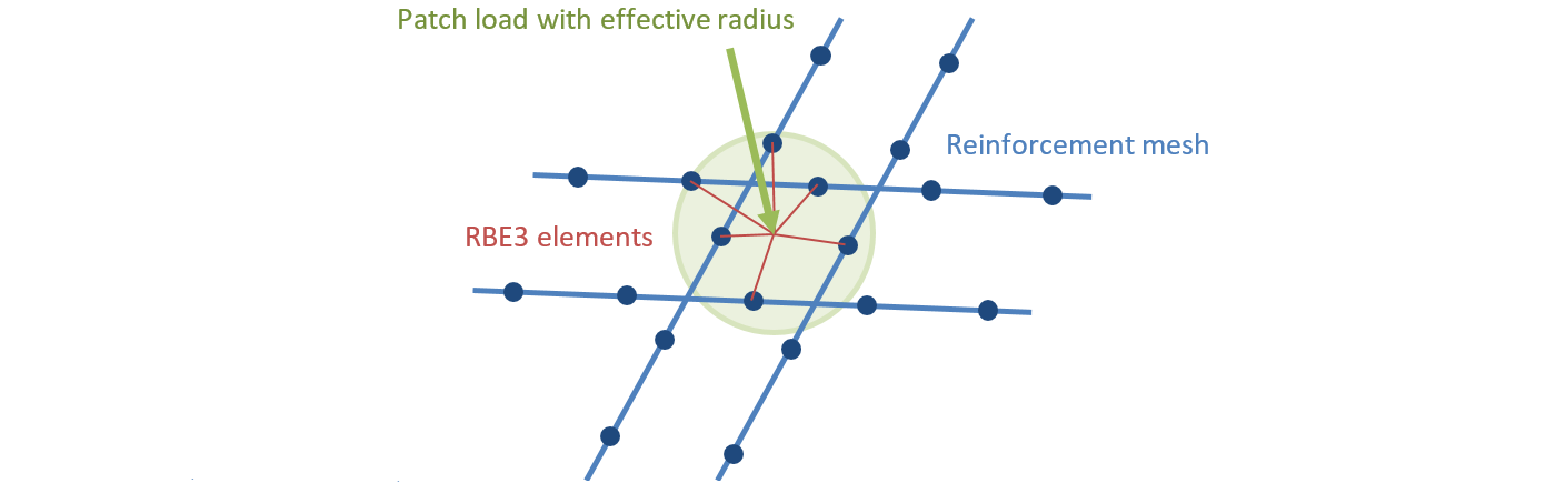
\[ \textsf{\textit{\footnotesize{Fig. 16\qquad Patch load mapping to reinforcement mesh.}}}\]

A vonalmenti támaszok és vonalmenti terhek a megadott szélesség vagy hatékony sugár alapján RBE3 elemekkel kapcsolódnak a betonháló csomópontjaihoz. A kapcsolatok súlya fordítottan arányos a támasztól vagy teherimpulzustól való távolsággal.

Az egyes terhek és a háló közötti kapcsolatról bővebben olvashat a Detail alkalmazás teherimpulzusainak általános leírásában

2.7 Megoldási módszer és terhelésszabályozási algoritmus

A nemlineáris végeselem-feladat megoldásához standard teljes Newton-Raphson (NR) algoritmust alkalmazunk.

Általában az NR algoritmus nem konvergál, ha a teljes terhelést egyetlen lépésben alkalmazzák. A szokásos megközelítés – amelyet itt is alkalmazunk – az, hogy a terhelést több lépésben, fokozatosan visszük fel, és az előző terhelési lépés eredményét használjuk kiindulópontként a következő Newton-megoldáshoz. Erre a célra egy terhelésszabályozási algoritmust implementáltunk a Newton-Raphson módszer fölé. Amennyiben az NR iterációk nem konvergálnak, az aktuális terhelési lépést felére csökkentjük, és az NR iterációkat megismételjük.

A terhelésszabályozási algoritmus második célja a kritikus terhelés meghatározása, amely bizonyos „leállási feltételeknek" felel meg – konkrétan a beton maximális alakváltozásának, a kötési elemekben fellépő maximális csúszásnak, a horgonyzási elemekben fellépő maximális elmozdulásnak és a betonacél-rudak maximális alakváltozásának. A kritikus terhelést felezési módszerrel határozzuk meg. Amennyiben a leállási feltétel a modell bármely pontján teljesül, az utolsó terhelési lépés eredményeit elvetjük, és az előző lépés felének megfelelő új lépést számítunk. Ezt a folyamatot addig ismételjük, amíg a kritikus terhelést egy meghatározott hibahatáron belül meg nem találjuk.

Beton esetén a leállási feltételt nyomásban 5%-os alakváltozásra (azaz a beton tényleges tönkremeneteli alakváltozásánál körülbelül egy nagyságrenddel nagyobb értékre), húzásban pedig a héjelemek integrációs pontjaiban 7%-os alakváltozásra állítottuk be. Húzásban az értéket úgy választottuk meg, hogy a vasalás határalakváltozása – amely a húzási merevítő hatás figyelembevétele nélkül általában kb. 5% – elsőként érhető el. Nyomásban az értéket több alternatíva közül úgy választottuk ki, hogy elég nagy legyen ahhoz, hogy a zúzódás hatásai láthatók legyenek az eredményekben, ugyanakkor elég kis ahhoz, hogy ne okozzon túl sok numerikus stabilitási problémát.

\[ \textsf{\textit{\footnotesize{Fig. 17\qquad Constitutive relationship of bond and anchorage elements used for anchorage length verification:}}}\]

\[ \textsf{\textit{\footnotesize{(a) bond shear stress slip response of a bond element; (b) force-displacement response of an anchorage element.}}}\]

Vasalás esetén a leállási feltétel feszültségek alapján van meghatározva. Mivel a repedésben ébredő feszültségeket modellezzük, a húzási feltétel a biztonsági tényezőt figyelembe vevő vasalás húzószilárdsságának felel meg. Ugyanezt az értéket alkalmazzuk a nyomási feltételre is.

A kötési elemekben és horgonyzási rugókban a leállási feltétel α·δu_max, ahol δu_max a szabványellenőrzésekben alkalmazott maximális csúszás, és α = 10.

2.8 Eredmények bemutatása

Az eredmények a beton és a vasalási elemek esetében külön-külön kerülnek bemutatásra. A betonban ébredő feszültség- és alakváltozás-értékeket a héjelemek integrációs pontjaiban számítják. Mivel azonban az adatok ilyen formában történő megjelenítése nem praktikus, az eredmények alapértelmezés szerint csomópontokban kerülnek bemutatásra, például a szomszédos Gauss-integrációs pontokból a kapcsolódó elemekben vett maximális nyomófeszültség értékeként (18. ábra). Meg kell jegyezni, hogy ez a megjelenítési mód helyileg alábecsülheti az eredményeket a szerkezeti elemek nyomott szélein, ha a végeselem mérete hasonló a nyomási zóna mélységéhez.

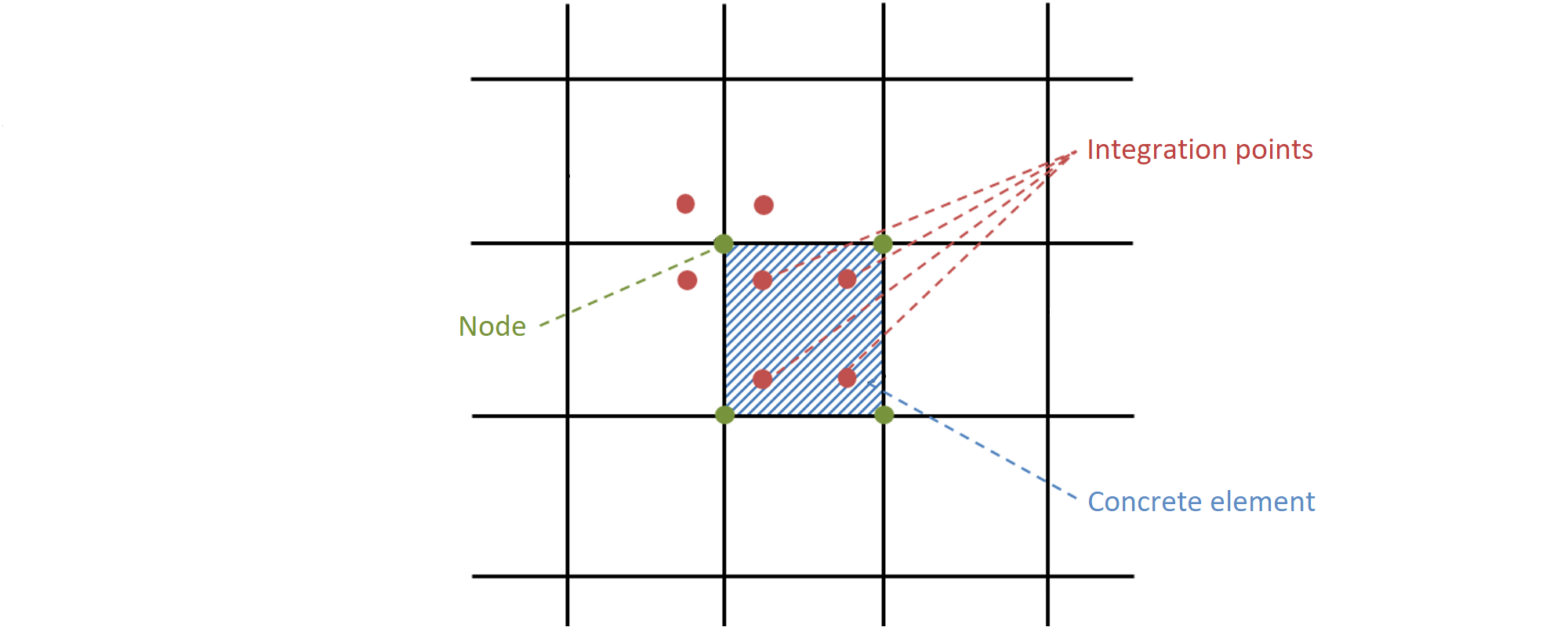
18. ábra – Beton végeselem integrációs pontokkal és csomópontokkal: az eredmények bemutatása betonra csomópontokban és végeselemekben.

A vasalási végeselemek eredményei elemenként vagy állandók (egy érték – pl. acélfeszültségek esetén), vagy lineárisak (két érték – tapadási eredmények esetén). A segédelemek, például az alátétlemezek elemei esetén csak az alakváltozások kerülnek bemutatásra.

3 Modell-ellenőrzés

3.1 Határállapotok és repedésszélesség-számítás

A szerkezet CSFM segítségével történő értékelése két különböző analízissel történik: egy a használhatósági, egy az teherbírási határállapoti teherkombinációkhoz. A használhatósági analízis feltételezi, hogy az elem teherbírási viselkedése kielégítő, és az anyag folyási feltételei nem érik el a használhatósági terhelési szinteken. Ez a megközelítés lehetővé teszi egyszerűsített anyagmodellek alkalmazását (a beton feszültség-alakváltozás diagram lineáris ágával) a használhatósági analízishez, a numerikus stabilitás és a számítási sebesség javítása érdekében. Ezért ajánlott az alább bemutatott munkafolyamat alkalmazása, amelyben a teherbírási határállapoti analízis az első lépésként kerül elvégzésre.

Teherbírási határállapoti analízis

Az egyes tervezési szabványok által előírt különböző ellenőrzések a modell által közvetlenül szolgáltatott eredmények alapján kerülnek értékelésre. A ULS ellenőrzések a beton szilárdsága, a vasalás szilárdsága és a lehorgonyzás (tapadási nyírófeszültségek) tekintetében kerülnek elvégzésre.

Annak érdekében, hogy egy szerkezeti elem hatékony méretezéssel rendelkezzen, erősen ajánlott egy előzetes analízis futtatása, amely az alábbi lépéseket veszi figyelembe:

Válassza ki a legkritikusabb teherkombinációk egy részét.
Csak a teherbírási határállapoti (ULS) teherkombinációkat számítsa.
Használjon durva hálót (az alapértelmezett hálóméret szorzójának növelésével a Beállításokban (19. ábra)).

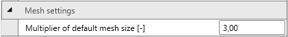
\[ \textsf{\textit{\footnotesize{Fig. 19\qquad Mesh multiplier.}}}\]

Egy ilyen modell nagyon gyorsan számít, lehetővé téve a tervezők számára, hogy hatékonyan áttekinthessék a szerkezeti elem részletezését, és újrafuttassák az analízist, amíg az összes ellenőrzési követelmény teljesül a legkritikusabb teherkombinációkra. Miután az előzetes analízis összes ellenőrzési követelménye teljesült, javasolt a teljes teherbírási teherkombinációk bevonása és finom hálóméret alkalmazása (a program által ajánlott hálóméret). A felhasználó a szorzóval módosíthatja a hálóméretet, amely 0,5-től 5-ig vehet fel értékeket (19. ábra).

Az alaperedmények és ellenőrzések (feszültség, alakváltozás és kihasználtság (azaz a számított érték/szabványból vett határérték), valamint a főfeszültségek iránya beton elemek esetén) különböző ábrázolásokkal jelennek meg, ahol a nyomás általában pirossal, a húzás kékkel van jelölve. A teljes szerkezet globális minimális és maximális értékei, valamint az egyes felhasználó által meghatározott részek minimális és maximális értékei is kiemelhetők. A program egy külön lapján speciális eredmények is megjeleníthetők, mint például tenzorértékek, a szerkezet alakváltozásai, valamint a vasalórudak húzási merevítő hatásának számításához használt vasalási arányok (effektív és geometriai). Ezenkívül a kiválasztott kombinációkhoz vagy teheresetekhez tartozó terhek és reakciók is megjeleníthetők.

Használhatósági határállapoti analízis

Az SLS ellenőrzések a feszültségkorlátozásra, a repedésszélességre és az alakváltozási határokra vonatkoznak. A feszültségek ellenőrzése beton és vasalás elemekben az alkalmazandó szabvány szerint történik, az ULS-hez meghatározotthoz hasonló módon.

A használhatósági analízis bizonyos egyszerűsítéseket tartalmaz a teherbírási határállapoti analízisnél alkalmazott anyagmodellekhez képest. Tökéletes tapadást feltételez, azaz a lehorgonyzási hossz használhatósági szinten nem kerül ellenőrzésre. Ezenkívül a beton nyomási feszültség-alakváltozás görbéjének plasztikus ága figyelmen kívül marad, míg a rugalmas ág lineáris és végtelen. Ezek az egyszerűsítések javítják a numerikus stabilitást és a számítási sebességet, és nem csökkentik a megoldás általánosságát, amennyiben a használhatósági szinten kapott anyagfeszültség-határok egyértelműen a folyási pontjuk alatt maradnak (ahogyan azt a szabványok előírják). Ezért a használhatósági analízishez alkalmazott egyszerűsített modellek csak akkor érvényesek, ha az összes ellenőrzési követelmény teljesül.

Repedésszélesség-számítás és húzási merevítő hatás

Repedésszélesség-számítás

A repedésszélességek kiszámításának két módja van – stabilizált és nem stabilizált repedezés. A szerkezet egyes részeiben a geometriai vasalási arány alapján dönthető el, hogy melyik repedésszámítási modellt kell alkalmazni (TCM a stabilizált repedezéshez és POM a nem stabilizált repedezési modellhez).

\( \textsf{\textit{\footnotesize{Fig. 20 \qquad Crack width calculation: (a) considered crack kinematics; (b) projection of crack kinematics into the principal}}}\) \( \textsf{\textit{\footnotesize{directions of the reinforcing bar; (c) crack width in the direction of the reinforcing bar for stabilized cracking; (d) cases with}}}\) \( \textsf{\textit{\footnotesize{local non-stabilized cracking regardless of the reinforcement amount; (e) crack width in the direction of the reinforcing bar}}}\)\( \textsf{\textit{\footnotesize{for non-stabilized cracking.}}}\)

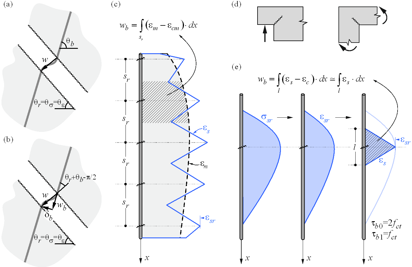
Míg a CSFM a legtöbb ellenőrzésnél közvetlen eredményt ad (pl. szerkezeti elem teherbírása, lehajlások…), a repedésszélesség-eredmények a végeselem-analízis által közvetlenül szolgáltatott vasalási alakváltozás-eredményekből kerülnek kiszámításra a 20. ábrán leírt módszertan szerint. Csúszás nélküli repedéskinematikát (tiszta repedésnyílás) veszünk figyelembe (20a. ábra), ami összhangban van a modell fő feltételezéseivel. A feszültségek és alakváltozások főirányai határozzák meg a repedések dőlésszögét (θ_r = θ_s= θ_e). A (20b. ábra) szerint a repedésszélesség (w) a vasalórud irányába vetíthető (w_b), ami a következőhöz vezet:

\[w = \frac{w_b}{\cos\left(θ_r + θ_b - \frac{π}{2}\right)}\]

ahol θ_b a rúd dőlésszöge.

Megjegyzendő, hogy a program θ_r és θ_b < π/2 értékeket jelenít meg. Ez azt jelenti, hogy az előző egyenlet olyan esetekre érvényes, ahol a vasalás és a repedés a Descartes-koordináta-rendszer különböző negyedein halad át, ahogy a 20. ábrán látható, ahol a vasalás az I. és III. negyeden, a repedés pedig a II. és IV. negyeden halad át. Azokban az esetekben, ahol a vasalás és a repedés ugyanazon negyedeken halad át, az egyenletet a következőképpen kell módosítani:

\[w = \frac{w_b}{\cos\left(-θ_r + θ_b + \frac{π}{2}\right)}\]

A w_b összetevő következetesen a húzási merevítő hatás modelljei alapján kerül kiszámításra a vasalási alakváltozások integrálásával. A teljesen kialakult repedésmintázattal rendelkező területeken a vasalórudak mentén számított átlagos alakváltozások (e_m) közvetlenül a repedéstávolság (s_r) mentén kerülnek integrálásra, ahogy a (20c. ábra) jelzi. Bár ez a repedési irányok kiszámítására vonatkozó megközelítés nem felel meg a repedések valós helyzetének, mégis reprezentatív értékeket ad, amelyek olyan repedésszélesség-eredményekhez vezetnek, amelyek összehasonlíthatók a szabvány által előírt repedésszélesség-értékekkel a vasalórud helyzetében.

Különleges helyzetek figyelhetők meg a számított szerkezet homorú sarkainál. Ebben az esetben a sarok előre meghatározza egyetlen repedés helyzetét, amely nem stabilizált módon viselkedik, mielőtt további szomszédos repedések alakulnának ki. Ezek a további repedések általában a használhatósági tartomány után alakulnak ki (Mata-Falcón 2015), ami indokolja, hogy az ilyen területen a repedésszélességeket úgy számítsák, mintha nem stabilizáltak lennének (21. ábra).

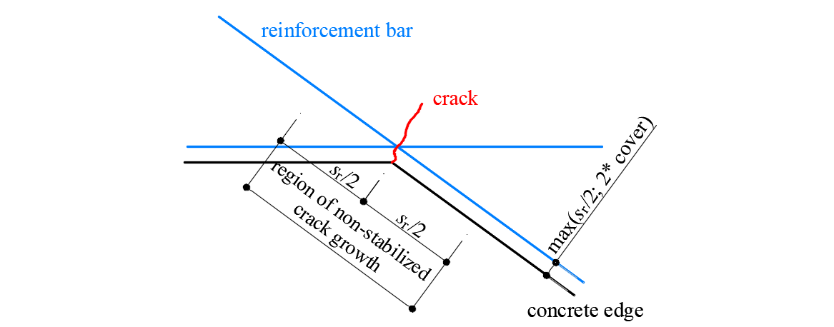
\[ \textsf{\textit{\footnotesize{Fig. 21\qquad Definition of the region at concave corners in which the crack width is computed as if it were non-stabilized.}}}\]

Húzási merevítő hatás

A húzási merevítő hatás implementációja különbséget tesz a stabilizált és nem stabilizált repedésmintázatok esetei között. Mindkét esetben a beton alapértelmezés szerint teljes mértékben repedezettnek tekintendő a terhelés előtt.

\( \textsf{\textit{\footnotesize{Fig. 22\qquad Tension stiffening model: (a) tension chord element for stabilized cracking with distribution of bond shear,}}}\) \( \textsf{\textit{\footnotesize{steel and concrete stresses, and steel strains between cracks, considering average crack spacing); (b) pull-out assumption}}}\) \( \textsf{\textit{\footnotesize{for non-stabilized cracking with distribution of bond shear and steel stresses and strains around the crack; (c) resulting}}}\) \( \textsf{\textit{\footnotesize{tension chord behavior in terms of reinforcement stresses at the cracks and average strains for European B500B steel;}}}\) \( \textsf{\textit{\footnotesize{(d) detail of the initial branches of the tension chord response.}}}\)

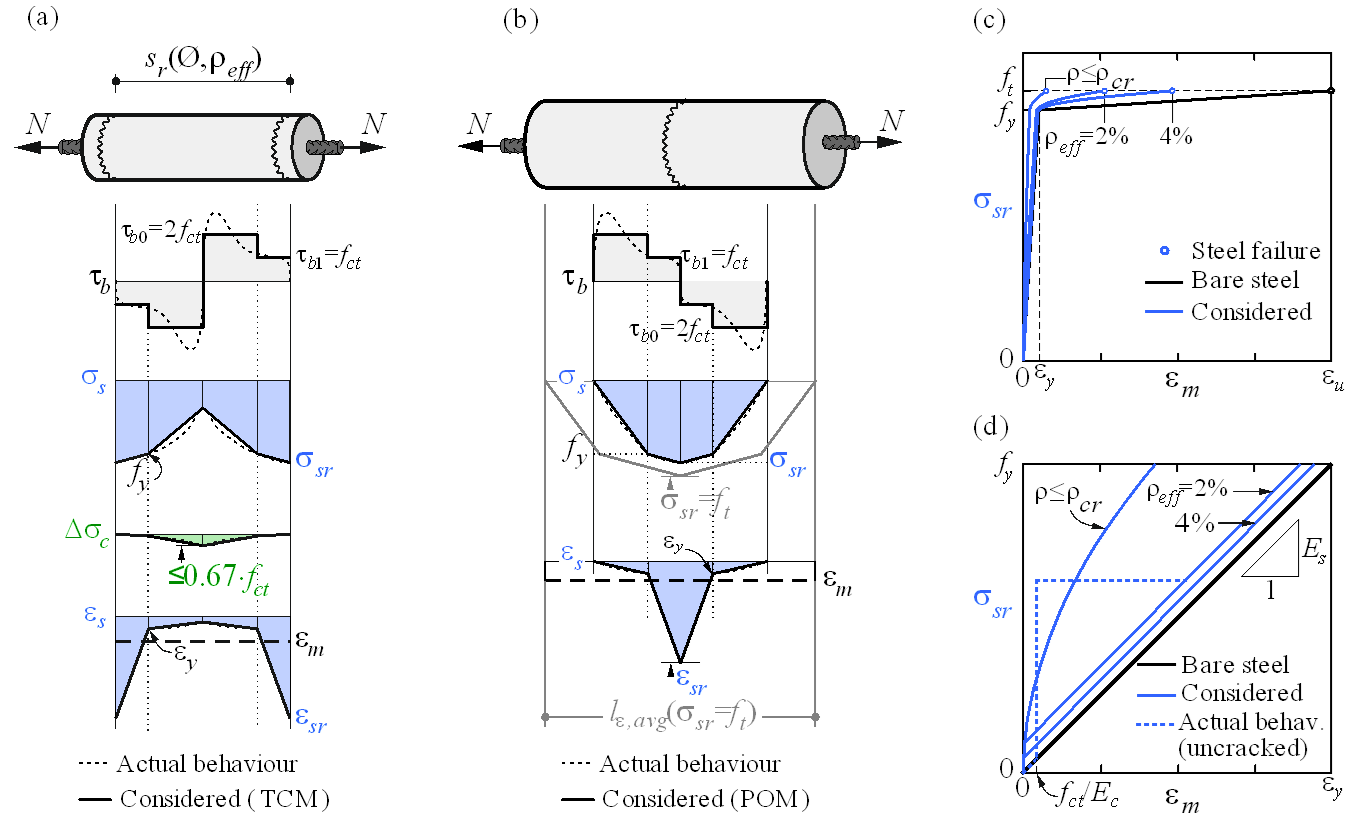
Stabilizált repedezés

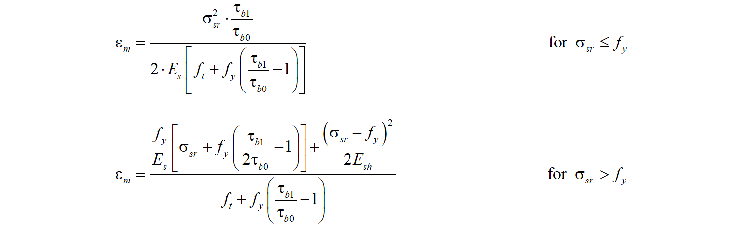
A teljesen kialakult repedésmintázatoknál a húzási merevítő hatás bevezetése a Tension Chord Model (TCM) segítségével történik (Marti et al. 1998; Alvarez 1998) – 22a. ábra –, amelyről kimutatták, hogy egyszerűsége ellenére kiváló válaszjóslatokat ad (Burns 2012). A TCM lépcsős, merev-tökéletesen képlékeny tapadási nyírófeszültség-csúszás összefüggést feltételez τ_b= τ_b₀ =2 f_ctm értékkel σ_s ≤ f_y esetén, és τ_b =τ_b₁ = f_ctm értékkel σ_s> f_y esetén. Minden vasalórudat húzott rudként kezelve – 22b. és 22a. ábra – a tapadási nyírás, az acél- és betonfeszültségek eloszlása, és ezáltal az alakváltozás-eloszlás két repedés között meghatározható az acél maximális feszültségeinek (vagy alakváltozásainak) bármely adott értékére a repedéseknél.

Az s_r = s_r₀ esetén új repedés keletkezhet vagy nem, mivel két repedés közötti középponton σ_c₁ = f_ct. Következésképpen a repedéstávolság kétszeres tényezővel változhat, azaz s_r = λs_r₀, ahol l = 0,5…1,0. Egy bizonyos λ értéket feltételezve a húzott rúd átlagos alakváltozása (ε_m) a maximális vasalási feszültségek (azaz a repedéseknél lévő feszültségek, σ_sr) függvényeként fejezhetőki. A CSFM-ben alapértelmezés szerint figyelembe vett idealizált bilineáris feszültség-alakváltozás diagramhoz a vasalórudak esetén a következő zárt alakú analitikus kifejezések adódnak (Marti et al. 1998):

\[\varepsilon_m = \frac{\sigma_{sr}}{E_s} - \frac{\tau_{b0}s_r}{E_s Ø}\]

\[\textrm{for}\qquad\qquad\sigma_{sr} \le f_y\]

\[{\varepsilon_m} = \frac{{{{\left( {{\sigma_{sr}} - {f_y}} \right)}^2}Ø}}{{4{E_{sh}}{\tau _{b1}}{s_r}}}\left( {1 - \frac{{{E_{sh}}{\tau_{b0}}}}{{{E_s}{\tau_{b1}}}}} \right) + \frac{{\left( {{\sigma_{sr}} - {f_y}} \right)}}{{{E_s}}}\frac{{{\tau_{b0}}}}{{{\tau_{b1}}}} + \left( {{\varepsilon_y} - \frac{{{\tau_{b0}}{s_r}}}{{{E_s}Ø}}} \right)\]

\[\textrm{for}\qquad\qquad{f_y} \le {\sigma _{sr}} \le \left( {{f_y} + \frac{{2{\tau _{b1}}{s_r}}}{Ø}} \right)\]

\[ \varepsilon_m = \frac{f_s}{E_s} + \frac{\sigma_{sr}-f_y}{E_{sh}} - \frac{\tau_{b1} s_r}{E_{sh} Ø}\]

\[\textrm{for}\qquad\qquad\left(f_y + \frac{2\tau_{b1}s_r}{Ø}\right) \le \sigma_{sr} \le f_t\]

ahol:
E_sh az acél keményedési modulusa E_sh = (f_t – f_y)/(ε_u – f_y /E_s) ,

E_s a vasalás rugalmassági modulusa,

Ø vasalórud átmérője,

s_rrepedéstávolság,

σ_sr vasalási feszültségek a repedéseknél,

σ_s   tényleges vasalási feszültségek,

f_ya vasalás folyáshatára.

Az IDEA StatiCa Detail CSFM-implementációja alapértelmezés szerint átlagos repedéstávolságot vesz figyelembe a számítógéppel segített feszültségmező-analízis elvégzésekor. Az átlagos repedéstávolságot a maximális repedéstávolság 2/3-ának tekintik (λ = 0,67), ami a hajlítási és húzási vizsgálatok alapján tett ajánlásokat követi (Broms 1965; Beeby 1979; Meier 1983). Megjegyzendő, hogy a repedésszélesség-számítások konzervatív értékek elérése érdekében maximális repedéstávolságot (λ = 1,0) vesznek figyelembe.

A TCM alkalmazása a vasalási aránytól függ, ezért döntő fontosságú az egyes vasalórudakhoz tartozó, repedések között húzásban dolgozó megfelelő betonterület hozzárendelése. Automatikus numerikus eljárást fejlesztettek ki a megfelelő hatékony vasalási arány (ρ_eff = A_s/A_c,eff) meghatározására bármely konfigurációhoz, beleértve a ferde vasalást is (23. ábra).

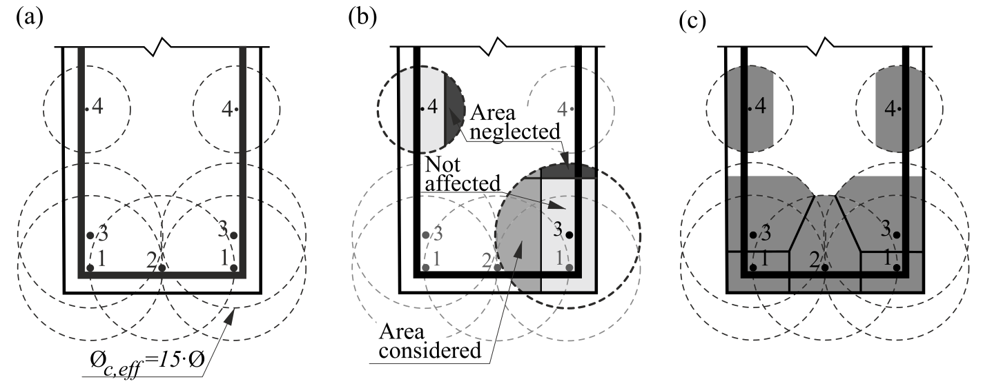
\( \textsf{\textit{\footnotesize{Fig. 23\qquad Effective area of concrete in tension for stabilized cracking: (a) maximum concrete area that can be activated;}}}\) \( \textsf{\textit{\footnotesize{(b) cover and global symmetry condition; (c) resultant effective area.}}}\)

Nem stabilizált repedezés

A ρ_cr-nél alacsonyabb geometriai vasalási arányú területeken lévő repedések – azaz a minimális vasalási mennyiség, amelynél a vasalás képes a repedési terhelést folyás nélkül felvenni – nem mechanikai hatások (pl. zsugorodás) vagy más vasalás által szabályozott repedések terjedése következtében keletkeznek. Ennek a minimális vasalásnak az értéke a következőképpen adódik:

\[{\rho _{cr}} = \frac{{{f_{ct}}}}{{{f_y} - \left( {n - 1} \right){f_{ct}}}}\]

ahol:

f_y a vasalás folyáshatára,

f_ct a beton húzószilárdsága,

n moduláris arány, n = E_s / E_c .

Hagyományos beton és vasalóacél esetén ρ_cr értéke körülbelül 0,6%.

A ρ_cr-nél alacsonyabb vasalási arányú kengyeleknél a repedezés nem stabilizáltnak tekintendő, és a húzási merevítő hatás a 22b. ábrán leírt Pull-Out Model (POM) segítségével kerül bevezetésre. Ez a modell egyetlen repedés viselkedését elemzi, figyelmen kívül hagyva az egyes repedések közötti mechanikai kölcsönhatást, elhanyagolva a beton húzási alakváltozhatóságát, és feltételezve a TCM által alkalmazott lépcsős, merev-tökéletesen képlékeny tapadási nyírófeszültség-csúszás összefüggést. Ez lehetővé teszi a vasalás alakváltozás-eloszlásának (ε_s) meghatározását a repedés közelében bármely maximális acélfeszültségre a repedésnél (σ_sr) közvetlenül az egyensúlyból. Tekintettel arra, hogy a repedéstávolság ismeretlen a nem teljesen kialakult repedésmintázat esetén, az átlagos alakváltozás (ε_m) bármely terhelési szinten a nulla csúszású pontok közötti távolságon kerül kiszámításra, amikor a vasalórud eléri húzószakítószilárdságát (f_t) a repedésnél (l_ε,_avg a 22b. ábrán), ami a következő összefüggésekhez vezet:

A javasolt modellek lehetővé teszik a tapadással rögzített vasalás viselkedésének kiszámítását, amelyet végül az analízisben figyelembe vesznek. Ez a viselkedés (beleértve a húzási merevítő hatást) a leggyakoribb európai vasalóacél esetén (B500B, f_t / f_y = 1,08 és ε_u = 5%) a 22c-d. ábrán látható.

4 Szerkezeti ellenőrzések Eurocode szerint

A szerkezet CSFM segítségével történő értékelése két különböző elemzéssel történik: egy a használhatósági, és egy a teherbírási határállapoti teherkombinációkhoz. A használhatósági elemzés feltételezi, hogy az elem teherbírási viselkedése kielégítő, és az anyag folyási feltételei nem érik el a használhatósági terhelési szinteken. Ez a megközelítés lehetővé teszi egyszerűsített anyagmodellek alkalmazását (a beton feszültség-alakváltozás diagram lineáris ágával) a használhatósági elemzéshez, a numerikus stabilitás és a számítási sebesség javítása érdekében.

4.1 Anyagmodellek (EN)

Beton - ULS

A CSFM-ben implementált betonmodell az EN 1992-1-1 által a keresztmetszetek méretezéséhez előírt egytengelyű nyomási alkotótörvényeken alapul, amelyek kizárólag a nyomószilárdságtól függnek. A CSFM alapértelmezés szerint az EN 1992-1-1 3.1.7 (1) bekezdésében meghatározott parabola-téglalap diagramot alkalmazza (24a. ábra), de a tervezők választhatják az EN 1992-1-1 3.1.7 (2) bekezdése szerinti egyszerűsített rugalmas-ideálisan képlékeny összefüggést is (24b. ábra). A húzószilárdságot elhanyagolják, ahogyan az a klasszikus vasbeton tervezésben is szokásos.

\[ \textsf{\textit{\footnotesize{Fig. 24\qquad The stress-strain diagrams of concrete for ULS: a) parabola-rectangle diagram; b) bilinear diagram.}}}\]

A CSFM IDEA StatiCa Detail-ben megvalósított változata nem alkalmaz explicit tönkremeneteli kritériumot a nyomott beton alakváltozásaira vonatkozóan (azaz a csúcsfeszültség elérése után 5% értékű ε_cu₂ (ε_cu₃) értékkel rendelkező képlékeny ágat vesz figyelembe, míg az EN 1992-1-1 0,35%-nál kisebb határalakváltozást feltételez). Ez az egyszerűsítés nem teszi lehetővé a nyomásban tönkremenő szerkezetek alakváltozási kapacitásának ellenőrzését. Ugyanakkor az EN 1992-1-1 3.1.3 szerinti f_cd teherbírási kapacitás megfelelően meghatározható, ha a repedezett beton tényezője (k_c₂, amelyet a 25. ábra definiál) mellett figyelembe veszik a beton ridegségének növekedését is a szilárdság emelkedésével, az fib Model Code 2010-ben az alábbiak szerint definiált \(\eta_{fc}\) redukciós tényező segítségével:

\[f_{cd}={\alpha_{cc}} \cdot \frac{f_{ck,red}}{γ_c} = {\alpha_{cc}} \cdot \frac{k_c \cdot f_{ck}}{γ_c} = {\alpha_{cc}} \cdot \frac{\eta _{fc} \cdot k_{c2} \cdot f_{ck}}{γ_c}\]

\[{\eta _{fc}} = {\left( {\frac{{30}}{{{f_{ck}}}}} \right)^{\frac{1}{3}}} \le 1\]

ahol:

α_cc a nyomószilárdságra gyakorolt hosszú távú hatásokat, valamint a teher alkalmazási módjából eredő kedvezőtlen hatásokat figyelembe vevő tényező. Az EN 1992-1-1 3.1.6 (1) bekezdése szerint értelmezendő. Alapértelmezett értéke 1,0.

k_ca nyomószilárdság globális redukciós tényezője

k_c₂ a keresztirányú repedések jelenlétéből adódó redukciós tényező

f_ck a beton hengeres karakterisztikus szilárdsága (MPa-ban megadva az \( \eta_{fc} \) definíciójához).

\[ \textsf{\textit{\footnotesize{Fig. 25\qquad The compression softening law.}}}\]

Beton - SLS

A használhatósági vizsgálat az ULS-elemzéshez alkalmazott alkotótörvények bizonyos egyszerűsítéseit tartalmazza. A beton nyomási feszültség-alakváltozás görbéjének képlékeny ága elhanyagolásra kerül, míg a rugalmas ág lineáris és végtelen. A nyomási lágyulás törvénye nem kerül figyelembevételre. Ezek az egyszerűsítések javítják a numerikus stabilitást és a számítási sebességet, és nem csökkentik a megoldás általánosságát, amennyiben a használhatósági állapotban kapott anyagfeszültségek egyértelműen a folyási határuk alatt maradnak (ahogyan azt az Eurocode megköveteli). Ezért a használhatósági vizsgálathoz alkalmazott egyszerűsített modellek csak akkor érvényesek, ha az összes ellenőrzési követelmény teljesül.

\[ \textsf{\textit{\footnotesize{Fig. 26\qquad Concrete stress-strain diagrams implemented for serviceability analysis: short- and long-term verifications.}}}\]

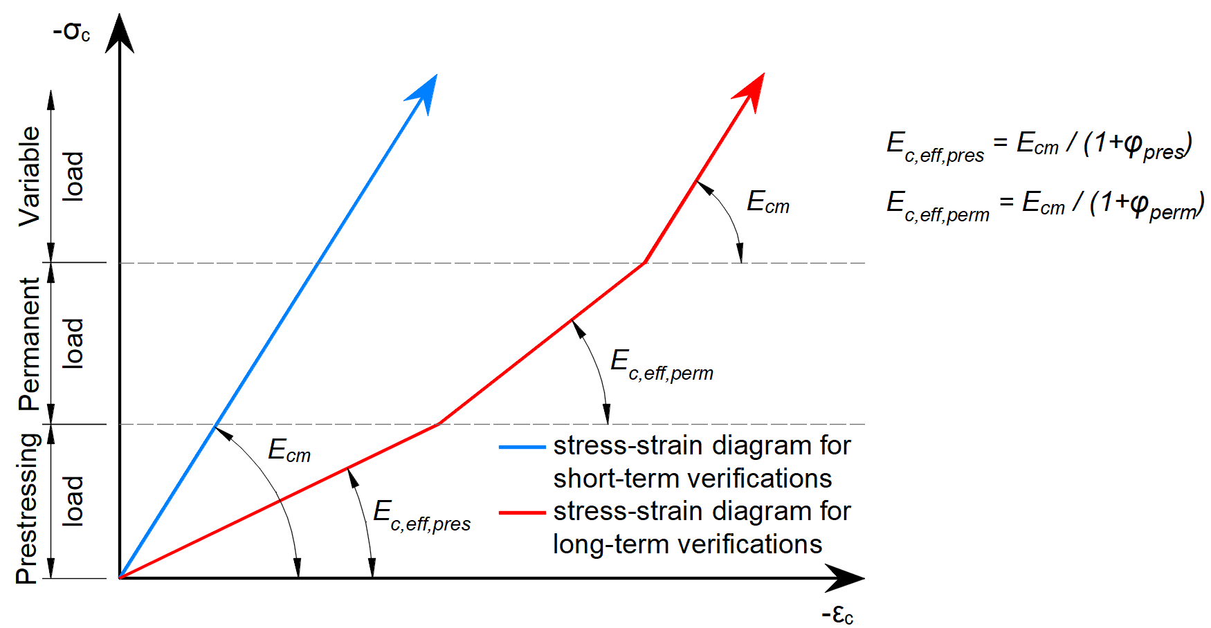
Hosszú távú hatások

A használhatósági vizsgálatban a beton hosszú távú hatásait egy effektív végtelen kúszási tényező (\(\varphi\), alapértelmezés szerint 2,5 értékkel) segítségével veszik figyelembe, amely az EN 1992-1-1 3.1.4 (3), illetve 7.4.3 (5) bekezdése szerint módosítja a beton szekansi rugalmassági modulusát (E_cm) az alábbiak szerint:

\[E_{c,eff} = \frac{E_{cm}}{1+\varphi}\]

A hosszú távú hatások figyelembevételekor először az összes állandó terhet tartalmazó teherlépést számítják a kúszási tényező alkalmazásával (azaz a beton effektív rugalmassági modulusával, E_c,eff), majd a pótlólagos terheket a kúszási tényező nélkül számítják (azaz E_cm alkalmazásával). Emellett a rövid távú ellenőrzések elvégzéséhez egy másik számítást is végeznek, amelyben az összes terhet a kúszási tényező nélkül számítják. A hosszú és rövid távú ellenőrzések mindkét számítása a 26. ábrán látható.

A kúszási tényezőket a felhasználó határozza meg az anyagtulajdonságokban, és azokat az EN 1992-1-1 3.1. ábra szerint kell meghatározni.

Vasalás

Alapértelmezés szerint az EN 1992-1-1 3.2.7 bekezdésében meghatározott, szabad betonacél rudakra vonatkozó idealizált bilineáris feszültség-alakváltozás diagramot alkalmazzák (27. ábra). E diagram meghatározásához csupán a vasalás alapvető tulajdonságainak ismerete szükséges a tervezési fázisban (szilárdság és képlékenységi osztály). Ha ismert, a vasalás tényleges feszültség-alakváltozás összefüggése (melegen hengerelt, hidegen alakított, edzett és önedzett stb.) is figyelembe vehető. A vasalás feszültség-alakváltozás diagramját a felhasználó is meghatározhatja, azonban ebben az esetben nem vehető figyelembe a húzási merevítő hatás (nem számítható a repedésszélesség). A vízszintes felső ággal rendelkező feszültség-alakváltozás diagram alkalmazása nem teszi lehetővé a szerkezeti tartósság ellenőrzését. Ezért a szabványos képlékenységi követelmények kézi ellenőrzése szükséges.

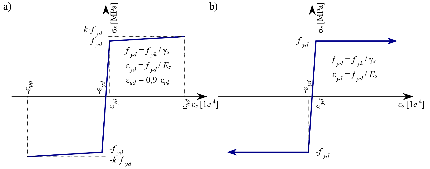
\( \textsf{\textit{\footnotesize{Fig. 27 \qquad Stress-strain diagram of reinforcement: a) bilinear diagram with an inclined top branch; b) bilinear diagram}}}\) \( \textsf{\textit{\footnotesize{with a horizontal top branch.}}}\)

A húzási merevítő hatás (28. ábra) automatikusan figyelembevételre kerül a szabad betonacél rúd bemeneti feszültség-alakváltozás összefüggésének módosításával, hogy megragadja a betonba ágyazott rudak átlagos merevségét (ε_m).

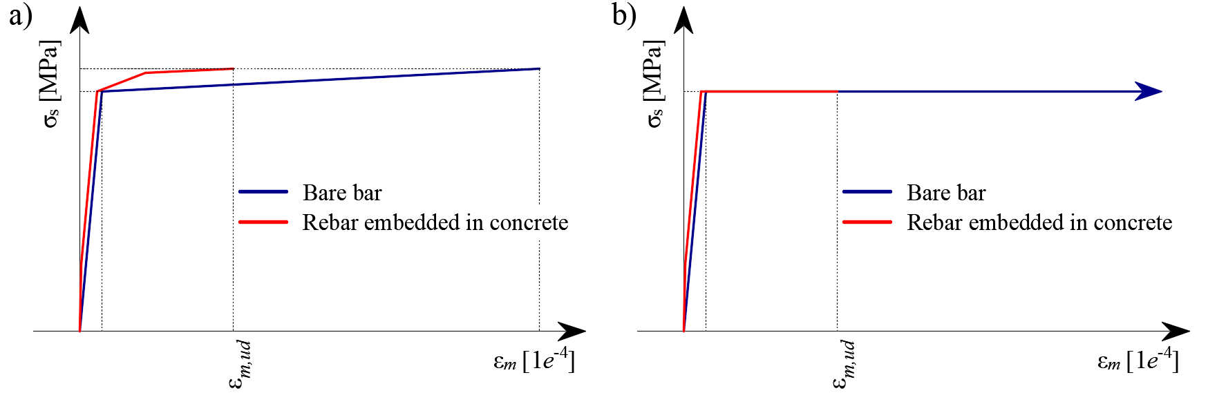
\[ \textsf{\textit{\footnotesize{Fig. 28\qquad Scheme of tension stiffening.}}}\]

4.2 Biztonsági tényezők

A Compatible Stress Field Method megfelel a modern tervezési szabványoknak. Mivel a számítási modellek csak szabványos anyagtulajdonságokat alkalmaznak, a tervezési szabványokban előírt részleges biztonsági tényező formátum minden módosítás nélkül alkalmazható. Ily módon a bemeneti terhek szorzófaktorral vannak ellátva, a jellemző anyagtulajdonságokat pedig a tervezési szabványokban előírt biztonsági együtthatókkal csökkentik, pontosan úgy, mint a hagyományos betonszerkezeti számításokban. Az EN 1992-1-1 2.4.2.4 fejezetében előírt anyagbiztonsági tényezők értékei alapértelmezettként vannak beállítva, de a felhasználó módosíthatja a biztonsági tényezőket a Szabvány és számítási beállításokban (29. ábra).

\[ \textsf{\textit{\footnotesize{Fig. 29\qquad The setting of material safety factors in Idea StatiCa Detail.}}}\]

A teherbiztonsági tényezőket a felhasználónak kell meghatároznia a Kombinációs szabályokban minden egyes nemlineáris teherkombinációhoz (30. ábra). Az Idea StatiCa Detail-ban megvalósított összes sablonhoz a részleges biztonsági tényezők már előre meg vannak határozva.

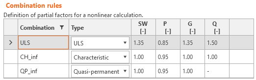
\[ \textsf{\textit{\footnotesize{Fig. 30\qquad The setting of load partial factors in Idea StatiCa Detail.}}}\]

A részleges biztonsági tényezők megfelelő, felhasználó által meghatározott kombinációinak alkalmazásával a felhasználók a CSFM segítségével a globális ellenállási tényező módszerrel is számíthatnak (Navrátil és mtsai, 2017), azonban ez a megközelítés a tervezési gyakorlatban alig használatos. Egyes irányelvek a nemlineáris analízishez a globális ellenállási tényező módszer alkalmazását javasolják. Ugyanakkor az egyszerűsített nemlineáris analízisekben (mint a CSFM), amelyek csak a hagyományos kézi számításokban használt anyagtulajdonságokat igénylik, még mindig előnyösebb a részleges biztonsági formátum alkalmazása.

4.3 Végső határállapot elemzés

Az EN 1992-1-1 által előírt különböző ellenőrzések a modell által közvetlenül szolgáltatott eredmények alapján kerülnek értékelésre. A ULS ellenőrzések a beton szilárdságára, a vasalás szilárdságára és a lehorgonyzásra (tapadási nyírófeszültségek) vonatkoznak.

A beton nyomási szilárdsága a végeselem-elemzésből kapott maximális főnyomófeszültség σ_c= σ_c₂ és a határérték σ_c,lim = f_cd arányaként kerül értékelésre.

A vasalás szilárdsága húzásban és nyomásban egyaránt a repedéseknél fellépő vasalási feszültség σ_sr és az előírt határérték σ_s,lim arányaként kerül értékelésre:

\(σ_{s,lim} = \frac{k \cdot f_{yk}}{γ_s}\qquad\qquad\textsf{\small{for bilinear diagram with inclined top branch}}\)

\(σ_{s,lim} = \frac{f_{yk}}{γ_s}\qquad\qquad\,\,\,\,\textsf{\small{for bilinear diagram with horizontal top branch}}\)

ahol:

f_yk a vasalás folyáshatára az EN 1992-1-1 3.2.3 cikk szerint,

k a húzószilárdság f_tk és a folyáshatár aránya,
\(k = \frac{f_{tk}}{f_{yk}}\)

γ_sa vasalás részleges biztonsági tényezője

A tapadási nyírófeszültség önállóan kerül értékelésre a végeselem-elemzéssel számított τ_b tapadási feszültség és az EN 1992-1-1 8.4.2 fejezet szerinti f_bd_, végső tapadási szilárdság arányaként:

\[\frac{τ_{b}}{f_{bd}}\]

\[f_{bd} = 2.25 \cdot η_1\cdot η_2\cdot f_{ctd}\]

ahol:

f_ctd a beton húzószilárdságának méretezési értéke az EN 1992-1-1 3.1.6 (2) cikk szerint. A magasabb szilárdságú betonok növekvő ridegségére tekintettel az f_ctk,0.05értéke az EN 1992-1-1 8.4.2 (2) cikk szerint C60/75 értékre van korlátozva

η₁ a tapadási feltételek minőségéhez és a betonozás közbeni betonacél-elhelyezkedéshez kapcsolódó együttható (31. ábra).

η₁ = 1,0 „jó" tapadási feltételek esetén, és

η₁ = 0,7 minden egyéb esetben, valamint csúszózsalus szerkezeti elemekben elhelyezett betonacélok esetén, kivéve ha igazolható, hogy „jó" tapadási feltételek állnak fenn

η₂ a betonacél átmérőjéhez kapcsolódó tényező:

η₂ = 1,0 Ø ≤ 32 mm esetén

η₂ = (132 - Ø)/100 Ø > 32 mm esetén

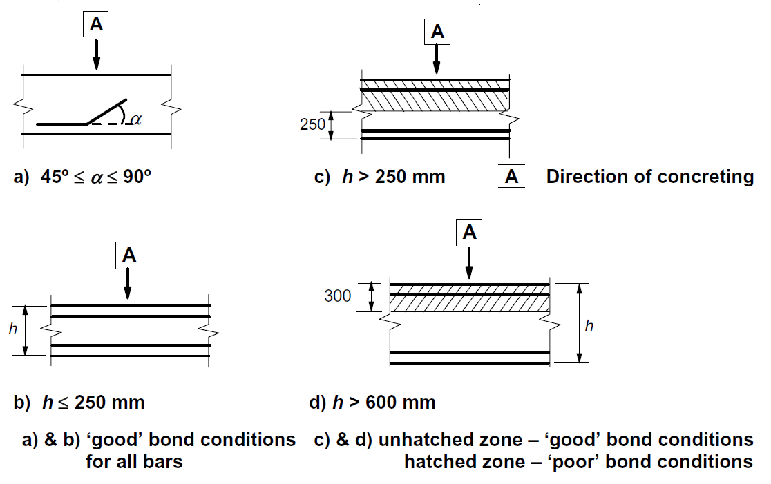
\[ \textsf{\textit{\footnotesize{Fig. 31\qquad EN 1992-1-1 Figure 8.2 - Description of bond conditions.}}}\]

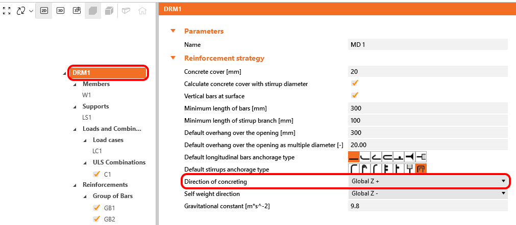
Az IDEA StatiCa Detail a tapadási feltételeket a 31. ábra c) és d) pontja szerint veszi figyelembe. A betonozás iránya az alkalmazásban minden egyes projektelemhez az alábbiak szerint állítható be.

Ezek az ellenőrzések a szerkezet egyes részeire vonatkozó megfelelő határértékek figyelembevételével kerülnek elvégzésre (azaz annak ellenére, hogy mind a beton, mind a vasalás anyagára egyetlen minőség van megadva, a végső feszültség-alakváltozás diagramok a szerkezet egyes részein eltérnek egymástól a húzási merevítő hatás és a nyomási lágyulás hatásai miatt).

Lehetőség van sima betonacélok modellezésére is. További információ itt található: Sima betonacélok a Detail-ban

Teljes erő F_tot és határerő F_lim

A teljes erő F_tot a végeselem-elemzés eredménye, és kétféleképpen definiálható.

\[F_{tot}=A_{s}\cdot \sigma_{s}\]

ahol A_s a betonacél keresztmetszeti területe és σ_s a betonacélban ébredő feszültség.

Vagy a lehorgonyzási erő F_aés a tapadási erő F_bond összegeként.

\[F_{tot}=F_{a}+F_{bond}\]

ahol F_a a lehorgonyzási rugóban ébredő tényleges erő, és F_bond a tapadási erő, amely a τ_b tapadási feszültség l hosszon való integrálásával kapható.

\[F_{bond}=C_{s} \cdot \int_{0}^{l}\tau_{b}\left( x \right)dx\]

C_s a betonacél kerülete.

A határerő F_lim a betonacél elemben ébredő maximális erő, figyelembe véve a betonacél végső szilárdságát és a lehorgonyzási feltételeket (tapadás a beton és a vasalás között, valamint lehorgonyzó horgok, hurkok stb.).

\[F_{lim}=min\left( F_{lim,bond}+F_{au},F_{u} \right)\]

\[F_{u}=k\cdot f_{yd}\cdot A_{s}\]

\[F_{au}=\beta\cdot k\cdot f_{yd}\cdot A_{s}\]

\[F_{lim,bond}=C_{s}\cdot l \cdot f_{bd}\]

ahol C_s a betonacél kerülete, és l a betonacél kezdetétől a vizsgált pontig mért hossz.

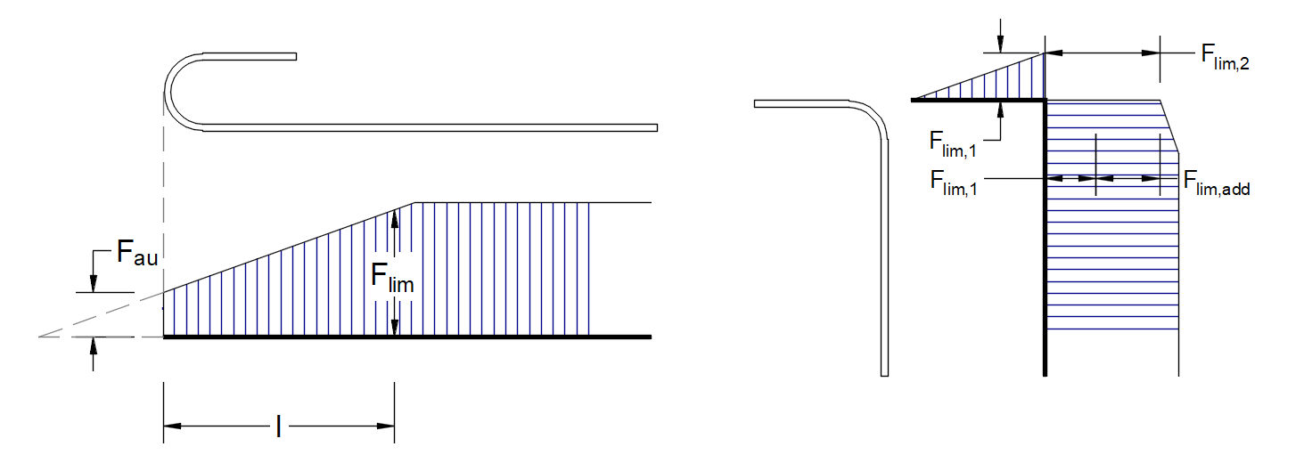
\[ \textsf{\textit{\footnotesize{Fig. 32\qquad Definition of the limit force Flim}}}\]

\[F_{lim,2}=F_{lim,1}+F_{lim,add}\]

ahol F_lim,add a szomszédos elemek közötti szög nagyságából számított pótlólagos erő. F_lim,2 mindig kisebb kell legyen, mint F_u.

A CSFM-ben elérhető lehorgonyzási típusok közé tartozik az egyenes betonacél (azaz lehorgonyzási hossz csökkentése nélkül), a hajlítás, a horog, a hurok, a hegesztett keresztirányú betonacél, a tökéletes tapadás és a folytonos betonacél. Mindezek a típusok a megfelelő β lehorgonyzási együtthatókkal együtt a 32. ábrán láthatók a hosszirányú vasalásra, a 33. ábrán pedig a kengyelekre vonatkozóan. Az alkalmazott lehorgonyzási együtthatók értékei az EN 1992-1-1 8.4.4 szakasz 8.2 táblázatával összhangban vannak. Megjegyzendő, hogy a különböző elérhető lehetőségek ellenére a CSFM háromféle lehorgonyzási véget különböztet meg: (i) a lehorgonyzási hossz csökkentése nélkül, (ii) a lehorgonyzási hossz 30%-os csökkentése normalizált lehorgonyzás esetén, és (iii) tökéletes tapadás.

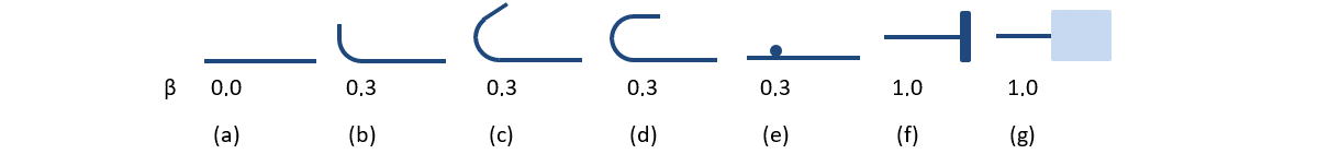
\[ \textsf{\textit{\footnotesize{Fig. 33\qquad Available anchorage types and respective anchorage coefficients for longitudinal reinforcing bars in the CSFM:}}}\]

\[ \textsf{\textit{\footnotesize{(a) straight bar; (b) bend; (c) hook; (d) loop; (e) welded transverse bar; (f) perfect bond; (g) continuous bar.}}}\]

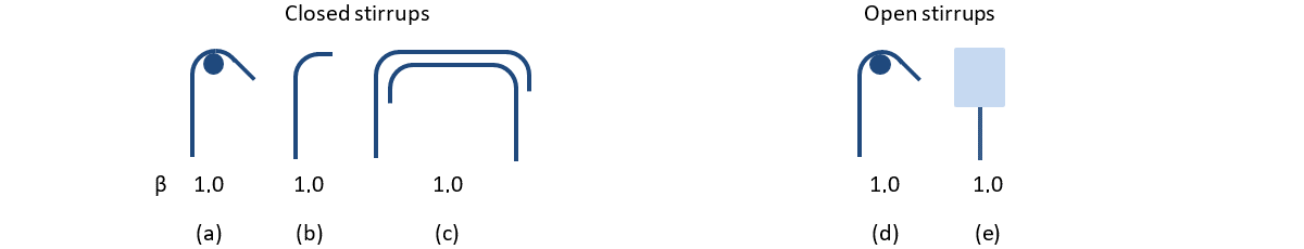
\[ \textsf{\textit{\footnotesize{Fig. 33\qquad Available anchorage types and respective anchorage coefficients for stirrups.}}}\]

\[ \textsf{\textit{\footnotesize{Closed stirrups: (a) hook; (b) bend; (c) overlap. Open stirrups: (d) hook; (e) continuous bar.}}}\]

Az EN 1992-1-1 követelményeinek való megfelelés érdekében a számításban a lehorgonyzási rugót kell alkalmazni; a lehorgonyzási rugót a β együttható módosítja, ezért a felhasználónak a vasalás kezdeti és végső feltételeinek meghatározásakor az elérhető lehorgonyzási típusok egyikét kell alkalmaznia.

4.4 Részlegesen terhelt területek (PLA)

Vasbeton szerkezetek tervezésekor a részlegesen terhelt területek (PLA) két nagy csoportjával találkozunk – az első csoportba a csapágyak, a másikba a lehorgonyzási területek tartoznak. A jelenleg érvényes vasbeton szerkezetek tervezésére vonatkozó EN 1992-1-1 szabvány 6.7. fejezete (34. ábra) szerint részlegesen terhelt területeknél figyelembe kell venni a beton helyi zúzódását és a keresztirányú húzóerőket. Egy A_c0 területen egyenletesen elosztott terhelés esetén a beton nyomási teherbírása a méretezési elosztási területtől (A_c1) függően akár háromszoros értékre is növelhető.

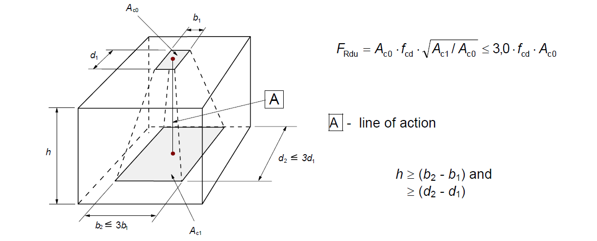
\[ \textsf{\textit{\footnotesize{Fig. 34\qquad Partially loaded areas according to EN 1992-1-1.}}}\]

A részlegesen terhelt területet megfelelő keresztirányú vasalással kell ellátni, amelyet a területen fellépő hasítóerők átvitelére kell méretezni. A részlegesen terhelt területek keresztirányú vasalásának méretezéséhez az Eurocode szerint a Strut-and-Tie módszert alkalmazzák. A szükséges keresztirányú vasalás nélkül nem lehet figyelembe venni a beton nyomási teherbírásának növekedését.

Részlegesen terhelt területek a CSFM-ben

\[ \textsf{\textit{\footnotesize{Fig. 35\qquad Fictitious struts with concrete finite element mesh.}}}\]

A CSFM alkalmazásával lehetőség van vasbeton szerkezetek tervezésére és ellenőrzésére, figyelembe véve a beton nyomási teherbírásának növekedését a részlegesen terhelt területeken. Mivel a CSFM egy síkbeli (2D) modell, a részlegesen terhelt területek pedig térbeli (3D) feladatot jelentenek, szükséges volt olyan megoldást találni, amely ezt a két különböző feladattípust ötvözi (35. ábra). Ha a „részlegesen terhelt területek" funkció aktiválva van, az Eurocode szerint létrejön a megengedett kúpgeometria (34. ábra). Az összes geometriai ütközés teljes mértékben 3D-ben kerül megoldásra az adott betonszerkezeti elem geometriájára és az egyes PLA-k méreteire vonatkozóan. Ezt követően elkészül a részlegesen terhelt terület számítási modellje.

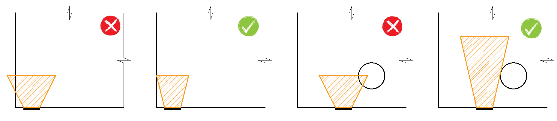
\[ \textsf{\textit{\footnotesize{Fig. 36\qquad Allowable cone geometries.}}}\]

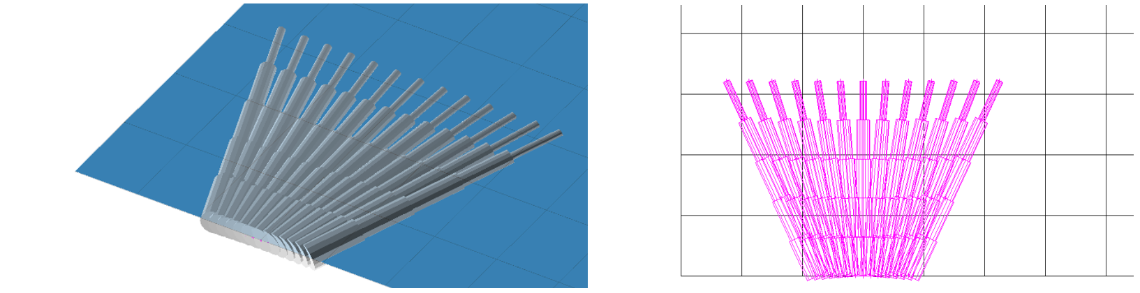
Az anyagmodell módosítása nem bizonyult megfelelő megközelítésnek, főként azért, mert a tulajdonságok végeselem-hálóra való leképezése problémás. Megállapítást nyert, hogy a végeselem-hálótól független megközelítés megfelelőbb megoldás. Az ismert nyomási kúpgeometriához teljesen koherens fiktív nyomott rudak jönnek létre (35. és 37. ábra). Ezek a rudak azonos anyagtulajdonságokkal rendelkeznek, mint a modellben alkalmazott beton, beleértve a feszültség-alakváltozás diagramot is. A kúp alakja határozza meg a rudak irányát, amelyek fokozatosan osztják el a terhelést a PLA-ról a méretezési elosztási területre. A fiktív rudak területsűrűsége a kúp egyes részein változó, és a terhelés irányában fiktív betonkeresztmetszetet ad hozzá. A terhelt terület szintjén (A_c0) a \(\sqrt{A_{c0} \cdot A_{c1}} - A_{real}\) aránynak megfelelő fiktív betonterület kerül hozzáadásra (ahol A_real a 2D számítási modellben feltételezett alátámasztás területe), és ez a terület lineárisan csökken nullára a méretezési elosztási terület (A_c1) felé. Ez a megoldás biztosítja, hogy a betonban ébredő nyomófeszültség állandó legyen a teljes kúptérfogaton.

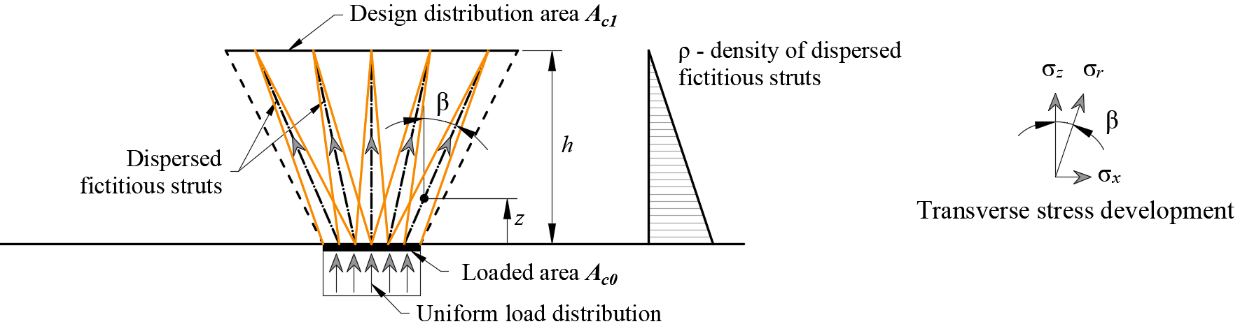
\[\rho \left( {\beta ,z} \right) = \left( {\sqrt {\frac{A_{c1}}{A_{c0}}} - \frac{A_{real}}{A_{c0}}} \right)\,\cdot\,\left( {1 - \frac{z}{h}} \right)\,\cdot\,\frac{1}{{\cos \beta }}\]

\[ \textsf{\textit{\footnotesize{Fig. 37\qquad Fictitious struts in the computational model}}}\]

A részlegesen terhelt terület teherbírása az EN 1992-1-1 (6.7) szerint a méretezési elosztási terület és a terhelt terület arányának megfelelően növekszik. Emlékeztetni kell arra, hogy ez egy méretezési modell, amely nem képes pontosan leírni a részlegesen terhelt terület feszültségállapotát, amelynek tényleges lefolyása jóval bonyolultabb. Ez a megoldás azonban lehetővé teszi a terhelés helyes elosztását a teljes modellre, miközben figyelembe veszi a részlegesen terhelt terület megnövelt teherbírását. Emellett helyesen vezeti be a keresztirányú feszültségeket ezen a területen.

A részlegesen terhelt területek funkció alkalmazásakor a beton nyomási teherbírásának növekedésének szimulálásához szükséges az EN 1992-1-1 6.7. szakasz (2) bekezdése szerinti szabványellenőrzés külön elvégzése. A vasalás által átvett keresztirányú húzóerők (hasítóerők) automatikusan ellenőrzésre kerülnek.

4.5 Használhatósági határállapot elemzés

Az SLS ellenőrzések a feszültségkorlátozásra, a repedésszélességre és az elhajláshatárokra vonatkoznak. A feszültségeket a betonban és a vasalási elemekben az EN 1992-1-1 szerint ellenőrzik, az ULS-hez meghatározotthoz hasonló módon.

Feszültségkorlátozás

A betonban lévő nyomófeszültséget korlátozni kell a hosszirányú repedések elkerülése érdekében. Az EN 1992-1-1 7.2 (2) fejezete szerint hosszirányú repedések keletkezhetnek, ha a jellemző teherkombináció alatti feszültségszint meghaladja a k₁f_ck értéket. A beton nyomási feszültsége a végeselem-elemzésből a használhatósági határállapotokra kapott maximális főnyomófeszültség σ_c = σ_c₂és a határérték σ_c,lim arányaként kerül meghatározásra. Ekkor:

\[\frac{σ_{c}}{σ_{c,lim}}\]

\[σ_{c,lim} = k_1\cdot f_{ck}\]

ahol:

f_ck a beton jellemző hengerszilárdága,

k₁ =0.6.

Ha a betonban a kvázi-állandó terhek alatt keletkező feszültség kisebb, mint k₂f_ck az EN 1992-1-1 7.2(3) cikk szerint, lineáris kúszás feltételezhető. Ha a betonban a feszültség meghaladja a k₂f_ck értéket, nemlineáris kúszást kell figyelembe venni (lásd EN 1992-1-1 3.1.4 cikk). Az IDEA StatiCa Detail programban csak az EN 1992-1-1 3.1.4 (3) cikk szerinti lineáris kúszás vehető figyelembe (lásd Anyagmodellek (EN)).

Feltételezhető, hogy nem megfelelő repedezés vagy alakváltozás elkerülhető, ha a jellemző teherkombináció alatt a vasalásban lévő húzófeszültség nem haladja meg a k₃f_yk értéket (EN 1992-1-1 7.2 (5) fejezet). A vasalás szilárdsága a repedéseknél fellépő vasalási feszültség σ_s = σ_sr és az előírt határérték σ_s,lim arányaként kerül meghatározásra:

\[\frac{σ_{s}}{σ_{s,lim}}\]

\[σ_{s,lim} = k_3\cdot f_{yk}\]

ahol:

f_yk a vasalás folyáshatára,

k₃ =0.8.

Elhajlás

Az elhajlások csak falak, illetve izostatikus (statikailag határozott) vagy hiperstatikus (statikailag határozatlan) gerendák esetén értékelhetők. Ezekben az esetekben az elhajlások abszolút értékét veszik figyelembe (a terhelés előtti kezdeti állapothoz képest), és az elhajlások maximálisan megengedhető értékét a felhasználónak kell megadnia. A levágott végeken az elhajlások nem ellenőrizhetők, mivel ezek lényegében instabil szerkezetek, ahol az egyensúlyt végső erők hozzáadásával biztosítják, ezért az elhajlások nem reálisak. A rövid távú u_z,st vagy hosszú távú u_z,lt elhajlás kiszámítható és ellenőrizhető a felhasználó által megadott határértékekkel szemben:

\[\frac{u_ z}{u_{z,lim}}\]

ahol:

u_z a végeselem-elemzéssel számított rövid vagy hosszú távú elhajlás,

u_z,lim a felhasználó által megadott elhajláshatárérték.

Repedésszélesség

A repedésszélességek és irányok csak hosszú távú hatásokra (az E_c,eff alkalmazásával) kerülnek kiszámításra azon kombinációkra, amelyeknél a repedésszélesség-ellenőrzés engedélyezett. Az Eurocode szerinti, felhasználó által megadott határértékeken alapuló ellenőrzések a következőképpen kerülnek bemutatásra:

\[\frac{w}{w_{lim}}\]

ahol:

w a végeselem-elemzéssel számított repedésszélesség,

w_lim a felhasználó által megadott repedésszélesség-határérték.

A repedésszélességek kiszámításának két módja van (stabilizált és nem stabilizált repedezés). Az általános esetben (stabilizált repedezés) a repedésszélesség a vasalórudak 1D elemeinek alakváltozásait integrálva kerül kiszámításra. A repedés iránya ezután az adott vasalás 1D végeseleméhez legközelebb eső (annak középpontjától mért) három integrációs pontból, a 2D betonelem integrációs pontjaiból kerül meghatározásra. Bár ez a repedési irányok kiszámítására alkalmazott megközelítés nem felel meg a repedések valós helyzetének, mégis reprezentatív értékeket ad, amelyek olyan repedésszélesség-eredményekhez vezetnek, amelyek összehasonlíthatók a szabvány által előírt repedésszélesség-értékekkel a vasalórud helyzetében.

5 Szerkezeti ellenőrzések ACI 318-19 szerint

A szerkezet CSFM segítségével történő értékelése két különböző elemzéssel történik: egy a használhatósági, és egy a teherbírási teherkombinációkhoz. A használhatósági elemzés feltételezi, hogy a tényezős terhek alatti viselkedés kielégítő, és az anyag folyási feltételei nem érik el a használhatósági terhelési szinteken. Ez a megközelítés lehetővé teszi egyszerűsített anyagmodellek alkalmazását (a beton feszültség-alakváltozás diagram lineáris ágával) a használhatósági elemzéshez, a numerikus stabilitás és a számítási sebesség javítása érdekében.

A CSFM megfelel az ACI 318-19, 6.8.1.1 fejezetének. Annak érdekében, hogy a CSFM teljesítse az ACI 318-19, 6.8.1.2 szakaszának követelményeit, számos ellenőrző vizsgálatot végeztek különböző egyetemeken. Az ellenőrzési és validálási eredményeket összefoglaló egyes cikkek az alábbi linken találhatók.

Ellenőrzések: Detail 2D

5.1 Anyagmodellek (ACI)

Beton - Szilárdság

A CSFM-ben a szilárdságszámításokhoz alkalmazott betonmodell a Portland Cement Association parabolikus feszültség-alakváltozás görbéjén alapuló parabolikus-képlékeny feszültség-alakváltozás diagramon alapul, amelyet a PCA's Notes on ACI 318-99 Building Code Requirements for Structural Concrete, 6-8. ábra tartalmaz. A húzószilárdságot elhanyagolják, ahogyan az a klasszikus vasbeton tervezésben is szokásos.

\[ \textsf{\textit{\footnotesize{Fig. 38\qquad The stress-strain diagram of concrete for Strength analysis}}}\]

Az IDEA StatiCa Detail CSFM-implementációja nem alkalmaz explicit tönkremeneteli kritériumot a nyomott beton alakváltozásaira vonatkozóan (azaz a csúcsfeszültség elérése után képlékeny ágat vesz figyelembe, ahol ε_c₀ maximális értéke 5%, míg az ACI 318-19 Cl. 22.2.2.1 szerint a határalakváltozás kisebb mint 0,3%). Ez az egyszerűsítés nem teszi lehetővé a nyomásban tönkremenő szerkezetek alakváltozási kapacitásának ellenőrzését. A szilárdság azonban megfelelően becsülhető, ha a repedezett beton tényezőjén (k_c₂, amelyet a (39. ábra) definiál) túlmenően a beton ridegségének szilárdság növekedésével arányos növekedését is figyelembe veszik a fib Model Code 2010-ben definiált \(\eta_{fc}\) redukciós tényező segítségével, az alábbiak szerint:

\[f'_{c,lim}=\alpha_{1}\cdot\phi_{c}\cdot k_{c}\cdot f'_{c}\]

\[k_{c}=\eta_{fc}\cdot k_{c2}\]

\[{\eta _{fc}} = {\left( {\frac{{30}}{{{f'_{c}}}}} \right)^{\frac{1}{3}}} \le 1\]

ahol:

α₁ a beton nyomószilárdsági redukciós tényezője, amelyet az ACI 318-19 Cl. 22.2.2.4.1 definiál. Parabola-téglalap feszültség-alakváltozás diagram alkalmazásakor a maximális nyomófeszültséget ezzel a tényezővel kell csökkenteni. Ez a nyomási zónában a feszültségeloszlást úgy átlagolja, hogy az eredő nyomószilárdság kisebb vagy egyenlő legyen a csökkenő képlékeny ággal rendelkező feszültség-alakváltozás diagram alapján számított nyomószilárdsággal.

Φ_ca beton szilárdsági redukciós tényezője. Az alapértelmezett értéket az ACI 318-19 Table 24.2.1 (b)(f) szerint kell meghatározni.

k_c₂ a keresztirányú repedések jelenlétéből adódó redukciós tényező.

f'_c a beton hengerszilárdága (MPa-ban megadva a \( \eta_{fc} \) definíciójához).

\[ \textsf{\textit{\footnotesize{Fig. 39\qquad The compression softening law.}}}\]

k_c₂ egy redukciós tényező, amely ugyanazon feltételezéseken alapul, mint az ACI 318-19 Table 23.9.2-ben megadott csomóponti zóna β_n együtthatója, azzal a különbséggel, hogy a CSFM-ben a főnyomási feszültségre merőleges főhúzási feszültség jelenlétét minden végeselem esetén ellenőrzik (nem csak a Strut and Tie modell csomópontjaiban).

Beton – Használhatóság

A használhatósági vizsgálat a szilárdságszámításhoz alkalmazott anyagmodellek bizonyos egyszerűsítéseit tartalmazza. A beton nyomási feszültség-alakváltozás görbéjének képlékeny ágát figyelmen kívül hagyják, míg a rugalmas ág lineáris és végtelen. A nyomási lágyulás törvényét nem veszik figyelembe. Ezek az egyszerűsítések javítják a numerikus stabilitást és a számítási sebességet, és nem csökkentik a megoldás általánosságát, amennyiben a használhatósági állapotban kapott anyagfeszültségek egyértelműen a folyáshatár alatt maradnak (ahogyan azt az ACI előírja). Ezért a használhatósági vizsgálathoz alkalmazott egyszerűsített modellek csak akkor érvényesek, ha minden ellenőrzési követelmény teljesül.

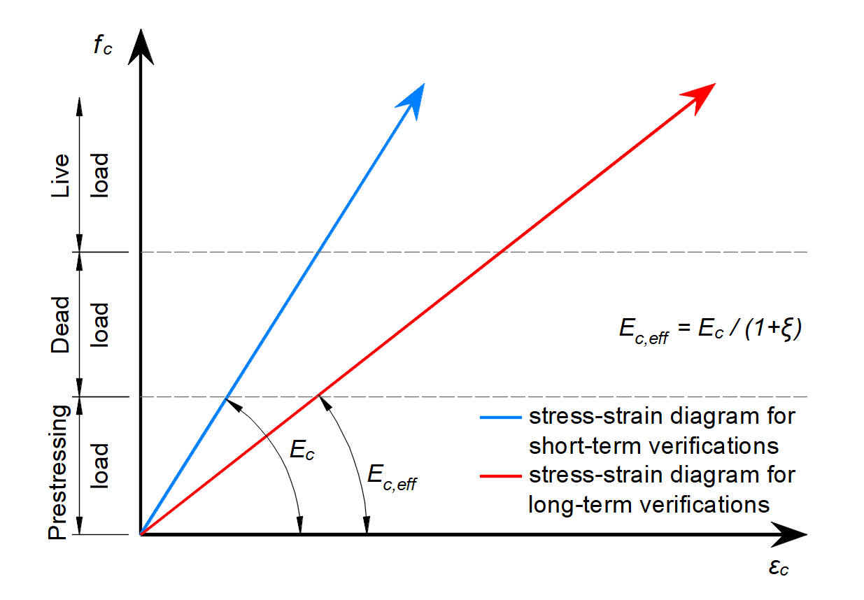
\[ \textsf{\textit{\footnotesize{Fig. 40\qquad Concrete stress-strain diagrams implemented for serviceability analysis: short- and long-term verifications.}}}\]

Hosszú távú hatások

A szerkezet hosszú távú viselkedését – mint például a hosszú távú lehajlásokat vagy a tartós terhek által okozott repedésszélességek számítását – a beton kúszása befolyásolja. Az ACI 318-19 24.2.4.1.3 bekezdése meghatározza a tartós terhekre vonatkozó időfüggő tényezőt – ξ –, amely az adott tartós terhelési időtartamra vonatkozó kúszási hatást fejezi ki.

A Detail alkalmazásban az E_c rugalmassági modulus a ξ tényező segítségével kerül módosításra a szerkezet hosszú távú viselkedésének meghatározásához. A módosított rugalmassági modulust E_c,eff-vel jelölik – lásd a 40. ábrát.

Feltéve, hogy az elem alakváltozása alakváltozással fejezhető ki, felírható, hogy:

\[\epsilon_{tot} = \epsilon_{0} + \epsilon_{creep} = \epsilon_{0} \cdot (1+\xi)\]

ahol:

ε₀ a rövid távú alakváltozás (kúszás hatása nélkül), és ε_creep a kúszás által okozott alakváltozás.

Hooke törvényét alkalmazva felírható:

\[E_{c,eff} = \frac{f_{c}}{\epsilon_{tot}}\]

Behelyettesítve \(\epsilon_{tot} = \epsilon_{0} \cdot (1+\xi)\) és \(\epsilon_{0} = f_{c} / E_{c}\) értékeket, kapjuk:

\[E_{c,eff} = \frac{E_{c}}{1+\xi}\]

A ξ tényező meghatározásához szükséges tartós terhelési időtartam minden egyes hosszú távú használhatósági kombinációhoz egyedileg beállítható.

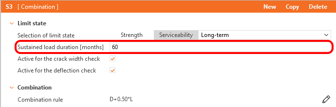
\[ \textsf{\textit{\footnotesize{Fig. 41\qquad Sustained load duration}}}\]

Az időfüggő lehajlásokat, feszültségeket és repedésszélességeket ezután egy módosított anyagmodellel számítják, amelyben a nyomási finomítás hatását a végeselem-analízis természete automatikusan figyelembe veszi. Ezért nem szükséges azokat tovább szorozni a 24.2.4.1.1-ben meghatározott tényezővel.

Rövid távú hatások

A rövid távú ellenőrzések elvégzéséhez egy másik számítást végeznek, amelyben minden terhet a tartós terhekre vonatkozó időfüggő tényező nélkül számítanak. A hosszú és rövid távú ellenőrzések mindkét számítása a 40. ábrán látható.

Vasalás

A nem feszített vasaláshoz tökéletesen rugalmas-képlékeny feszültség-alakváltozás diagramot alkalmaznak meghatározott folyáshatárral, lásd ACI 319-19 CL. 20.2.1. Ennek a diagramnak a meghatározásához csak a vasalás alapvető tulajdonságait kell ismerni – a szilárdságot és a rugalmassági modulust.

A vasalás feszültség-alakváltozás diagramját a felhasználó is meghatározhatja, azonban ebben az esetben nem lehet feltételezni a húzási merevítő hatást (nem lehet kiszámítani a repedésszélességet).

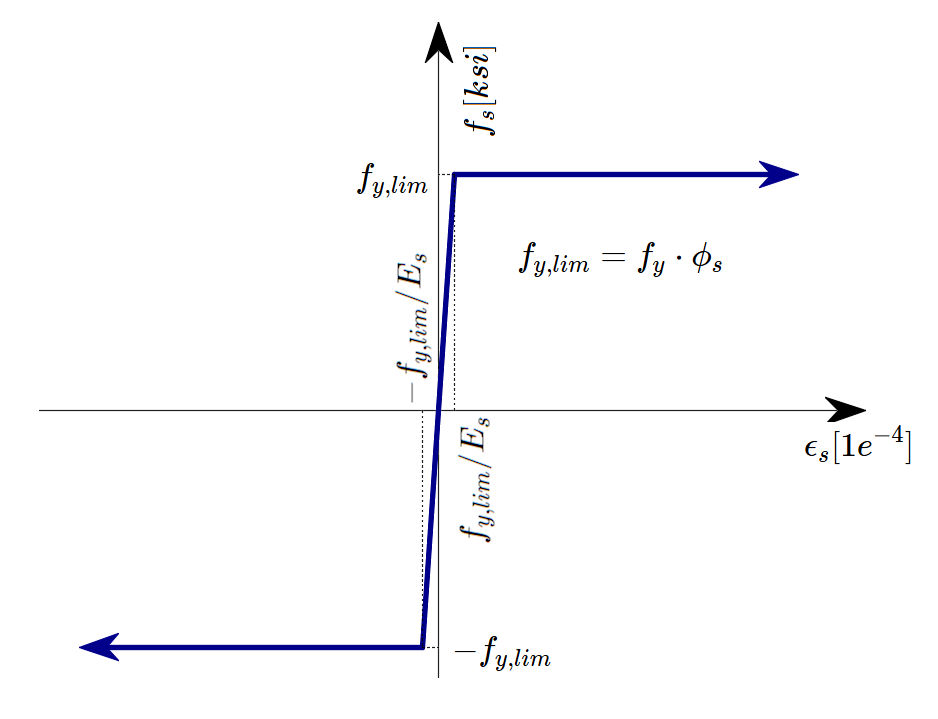
\[ \textsf{\textit{\footnotesize{Fig. 42 \qquad Stress-strain diagram of reinforcement}}}\]

ahol:

Φ_sa vasalás szilárdsági redukciós tényezője. Az alapértelmezett értéket az ACI 318-19 Table 24.2.1 szerint kell meghatározni.

f_y a vasalás folyáshatára

E_s a vasalás rugalmassági modulusa

10% van kiválasztva határalakváltozásként, amelynél a számítás leáll. Ez biztonságosnak tekinthető az ASTM A955/A955M-20c 7. cikke alapján.

A húzási merevítő hatást (43. ábra) automatikusan veszik figyelembe a szabad vasalórúd bemeneti feszültség-alakváltozás összefüggésének módosításával, hogy megragadják a betonba ágyazott rudak átlagos merevségét (ε_m).

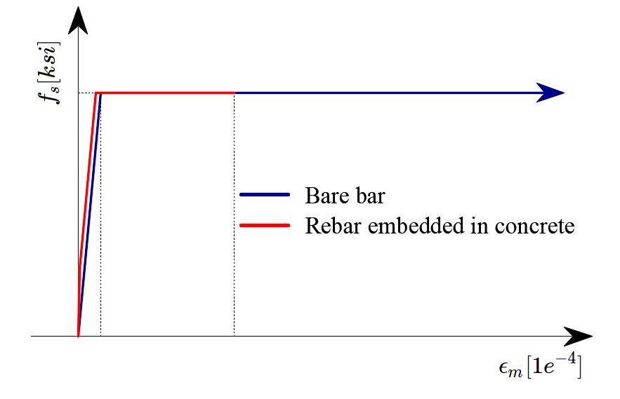
\[ \textsf{\textit{\footnotesize{Fig. 43\qquad Scheme of tension stiffening.}}}\]

5.2 Szilárdságcsökkentési és tehertényezők

A szilárdságcsökkentési tényezők értékeit az ACI 318-19 Cl. 21.2 írja elő. A beton és a vasalás alapértelmezett értékeit azon feltételezés alapján választják meg, hogy az alkalmazásban megoldott tipikus példa nyírásvezérelt (a 21.2.1 (b), (f), (g) táblázat alapján). Azonban bármilyen típusú szerkezeti elem modellezhető. Ezért, ha nyomás- vagy húzásvezérelt szerkezeti elemet vizsgálnak, a felhasználónak lehetősége van a szilárdságcsökkentési tényező értékét módosítani a Beállításokban.

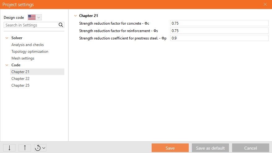
\[ \textsf{\textit{\footnotesize{Fig. 44\qquad The setting of strength reduction factors in IDEA StatiCa Detail.}}}\]

A Szilárdságkombinációkhoz tartozó tehertényezőket az ACI 318-19 5.3.1 táblázata szerint kell meghatározni.

A 34. fejezet rendelkezésein kívül a használhatósági szintű teherkombinációk nem kerülnek meghatározásra az ACI 318-19-ben. Javasolt az ASCE/SEI 7-16 C függeléke alapján meghatározott kombinációs szabályok alkalmazása. Minden sablonhoz a tehertényezők már előre meghatározottak.

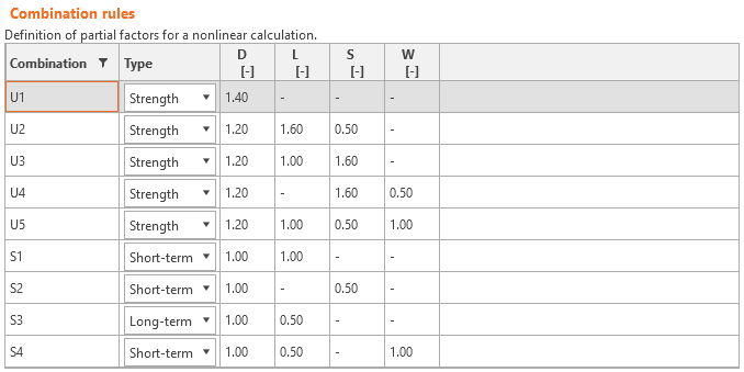
\[ \textsf{\textit{\footnotesize{Fig. 45\qquad The setting of load factors in Idea StatiCa Detail.}}}\]

5.3 Szilárdsági ellenőrzések

Az ACI 318-19 által előírt különböző ellenőrzések a modell által közvetlenül szolgáltatott eredmények alapján kerülnek értékelésre. Az ellenőrzések a beton szilárdsága, a vasalás szilárdsága és a lehorgonyzás (tapadási nyírófeszültségek) tekintetében kerülnek elvégzésre.

A beton szilárdsága nyomásban a végeselem-analízisből kapott maximális főnyomófeszültség f_c (más jelöléssel σ₂ a Kiegészítő eredményekben) és a határérték f'_c,lim arányaként kerül értékelésre.

A vasalás szilárdsága húzásban és nyomásban egyaránt a repedéseknél ébredő vasalási feszültség f_s és az előírt határérték f_y,lim arányaként kerül értékelésre.

A tapadási nyírófeszültség önállóan kerül értékelésre, mint a végeselem-analízissel számított τ_b tapadási feszültség és a f_bu tapadási szilárdság aránya.

Az ACI szabvány azonban nem foglalkozik közvetlenül a tapadási szilárdsággal, hanem az ún. lehorgonyzási hossz számításával dolgozik, amelyet a 25.4.2. szakasz ír le. Mivel a tapadási szilárdság a lehorgonyzási hossz meghatározásának alapvető bemeneti paramétere (lásd R25.4.1.1 és ACI Committee 408 1966), a tapadási szilárdság az alábbiak szerint számítható:

Tegyük fel, hogy ha a vasalásrudat betonba horgonyozzuk a l_d lehorgonyzási hosszig vagy annál nagyobb mértékben, a vasalás kihúzása a vasalás szakadásához vezet, nem pedig a betonból való kihúzódáshoz. Ez az alábbi képlettel írható fel.

\[\pi\cdot d_{b} \cdot l_{d} \cdot f_{bu}=f_{y}\cdot A_{s}\]

ahol:

d_b a vasalásrúd átmérője, l_d a lehorgonyzási hossz, f_bu a tapadási szilárdság, f_y a vasalás folyáshatára, és A_s a vasalásrúd keresztmetszetének területe.

A fentiekből a tapadási szilárdság számítási képlete könnyen levezethető:

\[f_{bu}=\frac{f_{y}\cdot A_{s}}{\pi\cdot d_{b} \cdot l_{d} }\]

A l_d lehorgonyzási hossz ezután az ACI 318-19 25.4.2.3 táblázata szerint az alábbiak szerint határozható meg:

\[l_{d}=\left( \frac{f_{y}\cdot\psi_{t}\cdot\psi_{e}\cdot\psi_{g}}{C\cdot\lambda\sqrt{f'_{c}}} \right)\cdot d_{b}\]

ahol:

C = 25 (metrikus rendszerben 2,1) a 6-os és kisebb átmérőjű betonacélokhoz és bordás huzalokhoz, C = 20 (metrikus rendszerben 1,7) a 7-es és nagyobb átmérőjű betonacélokhoz, λ = 1,0 normál súlyú beton esetén, ψ_t, ψ_e_, ψ_g az ACI 318-19 25.4.2.3 táblázata szerint kerülnek meghatározásra.

Csak bevonat nélküli vagy horganyzott (galvanizált) vasalás támogatott, ezért ψ_e = 1,0. ψ_g automatikusan kerül meghatározásra a vasalás minőségéből, és ψ_t automatikusan kerül levezetésre a vasalás modellbeli helyzetéből és a betonozás irányából, amely az alkalmazásban minden egyes projektelemhez az alábbiak szerint állítható be.

\[ \textsf{\textit{\footnotesize{Fig. 46\qquad Direction of concreting}}}\]

Lehetőség van sima betonacélok modellezésére is. További információ itt található: Sima betonacélok a Detail-ban

Teljes erő F_tot és határerő F_lim

A teljes erő F_tot a végeselem-analízis eredménye, és kétféleképpen definiálható.

\[F_{tot}=A_{s} \cdot f_{s}\]

ahol A_s a vasalásrúd keresztmetszetének területe és f_s a rúdban ébredő feszültség.

Vagy a lehorgonyzási erő F_aés a tapadási erő F_bond összegeként.

\[F_{tot}=F_{a}+F_{bond}\]

ahol F_a a lehorgonyzási rugóban ébredő tényleges erő, és F_bond a tapadási erő, amely a τ_b tapadási feszültség l vasalásrúd-hosszon való integrálásával kapható meg.

\[F_{bond}=C_{s} \cdot \int_{0}^{l}\tau_{b}\left( x \right)dx\]

C_s a vasalásrúd kerülete.

A határerő F_lim a betonacél elemben ébredő maximális erő, figyelembe véve a betonacél szilárdságát és a lehorgonyzási feltételeket (tapadás a beton és a vasalás között, valamint lehorgonyzó kampók, hurkok stb.).

\[F_{lim}=min\left( F_{lim,bond}+F_{au},F_{u} \right)\]

\[F_{u}=f_{y,lim}\cdot A_{s}\]

\[F_{au}=\beta\cdot f_{y,lim}\cdot A_{s}\]

\[F_{lim,bond}=C_{s}\cdot l \cdot f_{bu}\]

ahol C_s a vasalásrúd kerülete, és l a betonacél kezdetétől a vizsgált pontig mért hossz.

\[ \textsf{\textit{\footnotesize{Fig. 47\qquad Definition of the limit force Flim}}}\]

\[F_{lim,2}=F_{lim,1}+F_{lim,add}\]

ahol F_lim,add a szomszédos elemek közötti szög nagyságából számított pótlólagos erő. F_lim,2 mindig kisebb kell legyen, mint F_u.

A CSFM-ben elérhető lehorgonyzási típusok közé tartozik az egyenes rúd (azaz lehorgonyzási végi csökkentés nélkül), a 90 fokos kampó, a 180 fokos kampó, a tökéletes tapadás és a folytonos rúd. Mindezek a típusok, a megfelelő β lehorgonyzási együtthatókkal együtt, a 48. ábrán láthatók a hosszvasalás esetére. Az alkalmazott lehorgonyzási együtthatók értékei az ACI 318-19 25.4.3.1 szakaszából és az ACI 318-19 25.4.2.3 szakaszából vett egyenletek összehasonlításából kerülnek levezetésre. Megjegyzendő, hogy a különböző elérhető lehetőségek ellenére a CSFM háromféle lehorgonyzási véget különböztet meg: (i) a lehorgonyzási hossz csökkentése nélkül, (ii) a lehorgonyzási hossz 30%-os csökkentésével normalizált lehorgonyzás esetén, és (iii) tökéletes tapadás.

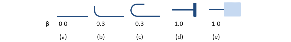
\[ \textsf{\textit{\footnotesize{Fig. 48\qquad Available anchorage types and respective anchorage coefficients for longitudinal reinforcing bars in CSFM:}}}\]

\[ \textsf{\textit{\footnotesize{(a) straight bar; (b) 90-degree hook; (c) 180-degree hook; (d) perfect bond; (e) continuous bar}}}\]

A kengyelek lehorgonyzási együtthatója mindig β = 1,0.

Az ACI előírásainak való megfelelés érdekében a számításban lehorgonyzási rugót kell alkalmazni; a lehorgonyzási rugót a β együttható módosítja, ezért a felhasználónak a vasalás kezdeti és végső feltételeinek meghatározásakor az elérhető lehorgonyzási típusok egyikét kell alkalmaznia.

5.4 Alátámasztási és lehorgonyzási zónák – Részlegesen terhelt területek

Betonszerkezetek tervezésekor a részlegesen terhelt területek (PLA) két nagy csoportjával találkozunk – az első csoportba az alátámasztások, a másikba a lehorgonyzási zónák tartoznak.

A vasbeton szerkezetek tervezésére vonatkozó jelenleg érvényes ACI 318-19 szabvány 22.8. fejezete szerint az alátámasztásoknál figyelembe kell venni a beton helyi zúzódását és a keresztirányú húzóerőket. Egyenletesen elosztott terhelés esetén az A_c1 területen a beton nyomási teherbírása legfeljebb kétszeresére növelhető a A_c2 méretezési elosztási területtől függően. Lásd az ACI 318-19 22.8.3.2. táblázatát.

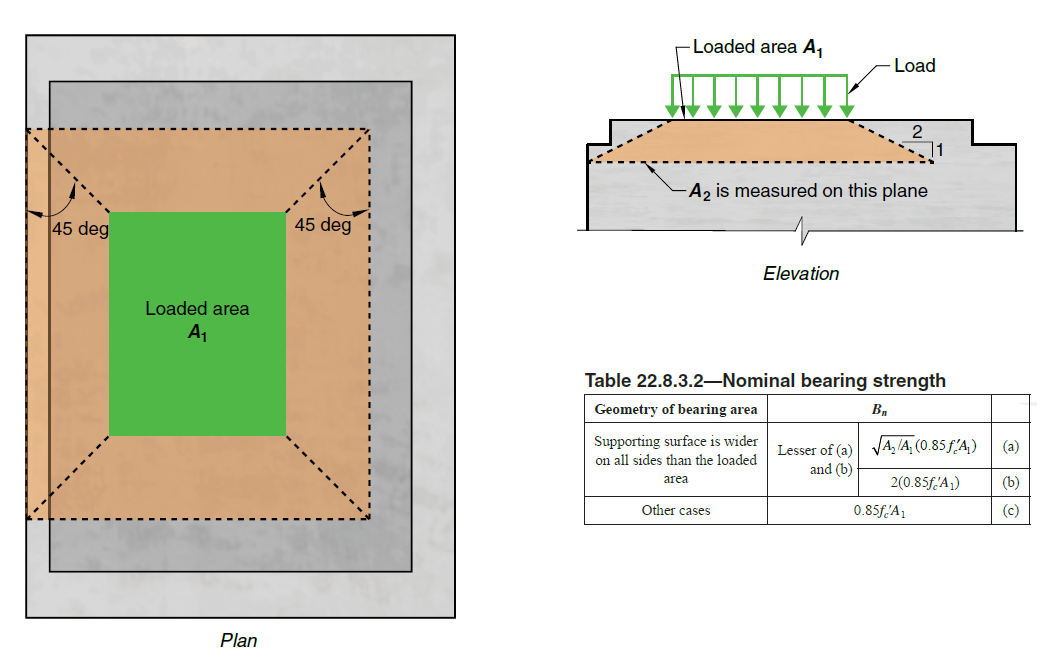
\[ \textsf{\textit{\footnotesize{Fig. 49\qquad Partially loaded areas for bearings according to ACI 318-19}}}\]

Az utófeszített lehorgonyzási zónák esetén az ACI 318-19 25.9. fejezetét kell követni.

A részlegesen terhelt területet megfelelő keresztirányú vasalással kell ellátni, amelyet a területen fellépő hasítóerők átvitelére kell méretezni. A szükséges keresztirányú vasalás nélkül nem vehető figyelembe a beton nyomási teherbírásának növekedése.

Részlegesen terhelt területek a CSFM-ben

\[ \textsf{\textit{\footnotesize{Fig. 50\qquad Fictitious struts with concrete finite element mesh.}}}\]

A CSFM alkalmazásával lehetőség van vasbeton szerkezetek tervezésére és ellenőrzésére, figyelembe véve a beton nyomási teherbírásának növekedését a részlegesen terhelt területeken. Mivel a CSFM egy síkbeli (2D) modell, a részlegesen terhelt területek pedig térbeli (3D) feladatot jelentenek, szükség volt egy olyan megoldás kidolgozására, amely ötvözi ezt a két különböző feladattípust (Fig. 50). Ha a „részlegesen terhelt területek" funkció aktiválva van, a megengedett kúpgeometria az ACI szerint kerül meghatározásra (Fig. 49). Az összes geometriai ütközés teljes mértékben 3D-ben kerül megoldásra az adott betonszerkezeti elem geometriájára és az egyes PLA-k méreteire vonatkozóan. Ezt követően elkészül a részlegesen terhelt terület számítási modellje.

\[ \textsf{\textit{\footnotesize{Fig. 51\qquad Allowable cone geometries.}}}\]

Az anyagmodell módosítása nem bizonyult megfelelő megközelítésnek, főként azért, mert a tulajdonságok végeselem-hálóra való leképezése problémás. Megállapítást nyert, hogy a végeselem-hálótól független megközelítés megfelelőbb megoldás. Az ismert nyomási kúpgeometriához teljesen koherens fiktív nyomott rudak kerülnek létrehozásra (Fig. 51 és Fig. 52). Ezek a rudak azonos anyagtulajdonságokkal rendelkeznek, mint a modellben alkalmazott beton, beleértve a feszültség-alakváltozás diagramot is. A kúp alakja határozza meg a rudak irányát, amelyek fokozatosan osztják el a terhelést a PLA-ról a méretezési elosztási területre. A fiktív rudak területsűrűsége változó a kúp egyes részein, és fiktív betonterületet ad hozzá a terhelés irányában. A terhelt terület szintjén (A_c1) a \(\sqrt{A_{c1} \cdot A_{c2}} - A_{real}\) aránynak megfelelő fiktív betonterület kerül hozzáadásra (ahol A_real a 2D számítási modellben feltételezett alátámasztás területe), és ez a terület lineárisan csökken nullára a méretezési elosztási terület (A_c2) felé. Ez a megoldás biztosítja, hogy a betonban lévő nyomófeszültség állandó legyen a teljes kúptérfogaton.

\[\rho \left( {\beta ,z} \right) = \left( {\sqrt {\frac{A_{c2}}{A_{c1}}} - \frac{A_{real}}{A_{c1}}} \right)\,\cdot\,\left( {1 - \frac{z}{h}} \right)\,\cdot\,\frac{1}{{\cos \beta }}\]

\[ \textsf{\textit{\footnotesize{Fig. 52\qquad Fictitious struts in the computational model}}}\]

A részlegesen terhelt terület teherbírása az ACI 318-19 22.8. fejezetében meghatározott méretezési elosztási terület és a terhelt terület arányának megfelelően növekszik. Emlékeztetni kell arra, hogy ez egy méretezési modell, amely nem képes pontosan leírni a részlegesen terhelt terület feszültségállapotát, amelynek tényleges lefolyása jóval bonyolultabb. Ez a megoldás azonban lehetővé teszi a terhelés helyes elosztását a teljes modellre, miközben figyelembe veszi a részlegesen terhelt terület megnövelt teherbírását. Emellett helyesen vezeti be a keresztirányú feszültségeket ezen a területen, hogy helyesen lehessen méretezni a hasítóerőkre a vasalást.

A megengedett alátámasztási feszültség 0,85f_c' értéke a 22.8.3.2. táblázatban szerepel. A sűrűség korlátozva van, hogy ne lépje túl a 22.8.3.2(b) táblázat képletében megadott maximális kétszeres teherbírást.

A lehorgonyzási zónák esetén a PLA ugyanúgy kerül alkalmazásra, mint az alátámasztásoknál. Ezért az ACI 318-19 25.9. fejezetében meghatározott helyi zónákat az ACI 318-19 25.9.3. pontja szerint manuálisan kell ellenőrizni. A PLA tehát csak arra szolgál, hogy elkerüljük az alakváltozási kritérium túllépését a helyi zónában, és ezáltal a számítás idő előtti leállását. Másrészt az ACI 318-19 25.9.4.3.1 (b) pontja szerint a síkbeli felhasadási és leválási feszültségeknek ellenálló vasalás közvetlenül és előnyösen ellenőrizhető az alkalmazásban.

5.5 Használhatósági ellenőrzések

A használhatósági ellenőrzések a feszültségkorlátozásra, a repedésszélességre és az elhajlási határértékekre vonatkoznak. A feszültségeket a betonban és a vasalási elemekben az ACI 318-19 szerint ellenőrzik, a Teherbíráshoz hasonló módon.

Feszültségkorlátozás

A használati terhelés melletti megengedett beton nyomófeszültségeket az U és T osztályú feszített szerkezeti elemeknél kell ellenőrizni. A R24.5.2.1 táblázat alapján a repedezettnek feltételezett betonnál nem szükséges feszültségkorlátozási ellenőrzés. A felhasználónak a tervezési szerkezeti elem beállításaiban meg kell adnia a feszített szerkezeti elem osztályát.

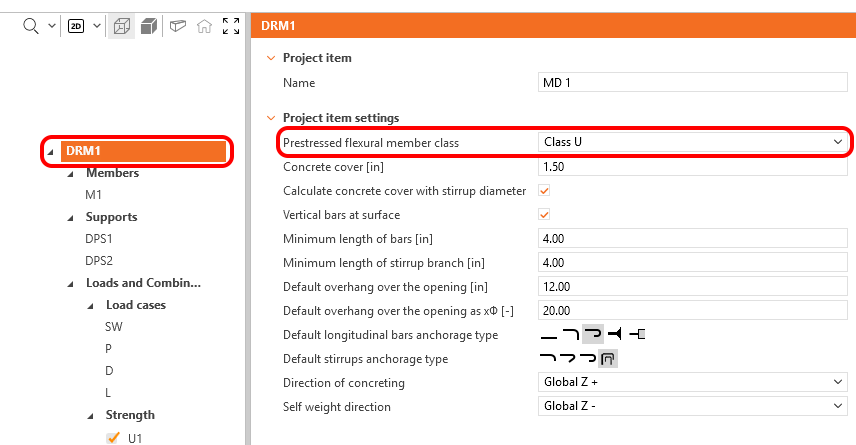
\[ \textsf{\textit{\footnotesize{Fig. 53\qquad Prestressed flexural member class selection}}}\]

Az átmeneti terhelésnek kitett szerkezeti elemek megengedett nyomófeszültsége az ACI 318-19 24.5.4.1 szerint 0,6f_c'. A 0,45f_c' nyomófeszültség-határértéket azért vezették be, hogy csökkentsék az ismétlődő terhelések miatti feszített betonszerkezeti elemek tönkremenetelének valószínűségét. Ez a határérték ésszerűnek tűnt a túlzott kúszási alakváltozás megelőzése szempontjából is. Magasabb feszültségértékeknél a kúszási alakváltozások az alkalmazott feszültség növekedésével egyre gyorsabban növekednek.

A beton nyomófeszültsége a végeselem-analízisből a használhatóságra kapott maximális főnyomófeszültség f_c = σ_c₂és a 24.5.4.1 táblázat alapján meghatározott határérték arányaként kerül kiértékelésre.

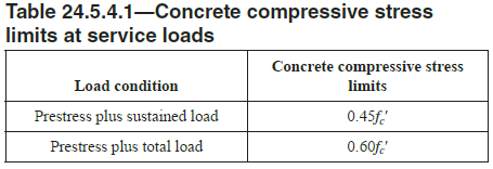
\[ \textsf{\textit{\footnotesize{Fig. 54\qquad Concrete compressive stress limits at service loads}}}\]

Az alkalmazásban az Előfeszítés és tartós terhelés hosszú távú kombinációként, az Előfeszítés és teljes terhelés rövid távú kombinációként kerül kezelésre.

Elhajlás

A kiválasztott kombinációtípustól (hosszú távú vagy rövid távú) függően hosszú távú vagy rövid távú elhajlás kerül kiértékelésre. A maximális megengedett elhajlási értéket a felhasználónak kell meghatároznia, és azt az ACI 138-19 24.2. pontjával összhangban kell figyelembe venni.

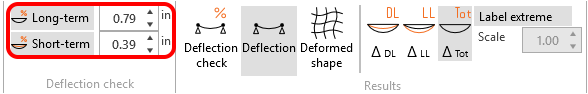
\[ \textsf{\textit{\footnotesize{Fig. 55\qquad Maximum allowable deflection value}}}\]

Az alkalmazásban lehetőség van az önsúlyból Δ_DL és a hasznos terhelésből Δ_LL származó elhajlások külön megjelenítésére, valamint a teljes elhajlás Δ_Tot(önsúly+hasznos) megjelenítésére, mindezt a deformált alak megjelenítésével együtt.

A levágott végeken az elhajlások nem ellenőrizhetők.

Repedésszélesség

A repedésszélességek és repedésirányok a használhatósági rövid távú vagy hosszú távú kombinációkra kerülnek kiszámításra. Mivel az ACI nem ír elő közvetlenül határértéket a repedésszélességre, a felhasználónak meg kell adnia a határrepedésszélességet w_lim.

Az ellenőrzések a következőképpen kerülnek bemutatásra:

\[\frac{w}{w_{lim}}\]

ahol:

w a végeselem-analízissel számított rövid vagy hosszú távú repedésszélesség,

w_lim a felhasználó által meghatározott repedésszélesség határértéke.

Az alkalmazásban használt repedésszélesség-számítási módszer, amelyet ez a dokumentum részletesebben is ismertet, az ACI 224R-01 szabványnak megfelelő. Ezért lehetséges az ACI 224R-01 4.1 táblázatának használata a repedésszélesség határértékének meghatározásához.

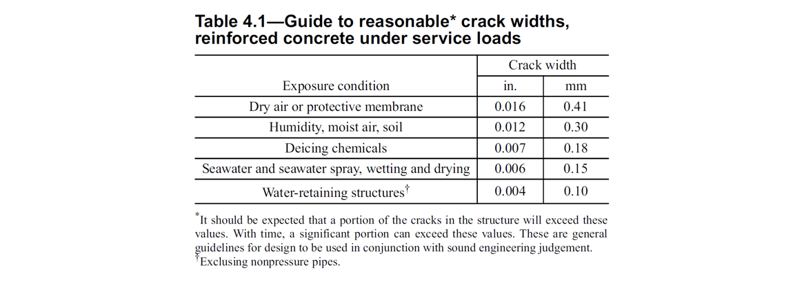
\[ \textsf{\textit{\footnotesize{Fig. 56\qquad Reasonable crack widths for reinforced concrete under service load}}}\]

A repedésszélesség kiszámításának két módja van (stabilizált és nem stabilizált repedezés). Az általános esetben (stabilizált repedezés) a repedésszélesség a vasalási rudak 1D elemeinek alakváltozásait integrálva kerül kiszámításra. A repedés iránya ezután az adott vasalás 1D végeselem középpontjához legközelebb eső három integrációs pontból, a 2D betonelem integrációs pontjaiból kerül meghatározásra. Bár ez a repedésirány-számítási megközelítés nem felel meg a repedések valós helyzetének, mégis reprezentatív értékeket ad, amelyek olyan repedésszélesség-eredményekhez vezetnek, amelyek összehasonlíthatók a szabvány által előírt repedésszélesség-értékekkel a vasalási rúd helyzetében.

6 Szerkezeti ellenőrzések AASHTO szerint

6.1 Anyagmodellek (AASHTO)

Beton - Teherbírás

A CSFM-ben a teherbírási számításokhoz implementált betonmodell az AASHTO LRFD egyensúlyi és alakváltozás-kompatibilitási feltételezésein alapul. Az AASHTO LRFD (2024) 5.6.2.1 cikke szerint a beton húzószilárdságát elhanyagolják.

\[ \textsf{\textit{\footnotesize{Fig. 57\qquad The stress-strain diagram of concrete for Strength analysis}}}\]

A CSFM implementációja az IDEA StatiCa Detail alkalmazásban nem vesz figyelembe explicit tönkremeneteli kritériumot az alakváltozások tekintetében nyomott beton esetén (azaz a csúcsfeszültség elérése után egy ε_c₀ maximálisan 5%-os értékű plasztikus ágat vesz figyelembe, míg az AASHTO LRFD (2024) 5.6.2.1 cikke 0,3%-nál kisebb végső alakváltozást feltételez). Ez az egyszerűsítés nem teszi lehetővé a nyomásban tönkremenő szerkezetek alakváltozási kapacitásának ellenőrzését. A teherbírás azonban megfelelően becsülhető, ha a repedezett beton tényezőjén (k_c₂, amelyet az (57. ábra) definiál) túlmenően a beton ridegségének növekedését – a szilárdság emelkedésével – az fib Model Code 2010-ben definiált \(\eta_{fc}\) redukciós tényező segítségével is figyelembe veszik:

\[f'_{c,lim}=\alpha_{1}\cdot\phi_{c}\cdot k_{c}\cdot f'_{c}\]

\[k_{c}=\eta_{fc}\cdot k_{c2}\]

\[{\eta _{fc}} = {\left( {\frac{{30}}{{{f'_{c}}}}} \right)^{\frac{1}{3}}} \le 1\]

ahol:

α₁ a beton nyomási szilárdságának redukciós tényezője, amelyet az AASHTO LRFD (2024) 5.6.2.2 cikke definiál. Parabola-téglalap feszültség-alakváltozás diagram alkalmazásakor a maximális nyomófeszültséget ezzel a tényezővel kell csökkenteni. Ez a nyomási zónában a feszültségeloszlást úgy átlagolja, hogy az eredő nyomási szilárdság kisebb vagy egyenlő legyen a csökkenő plasztikus ággal rendelkező feszültség-alakváltozás diagram alapján számított nyomási szilárdsággal.

Φ_ca beton ellenállási tényezője. Az alapértelmezett értéket az AASHTO LRFD (2024) 5.5.4.2 cikke szerint kell meghatározni.

k_c₂ a keresztirányú repedések jelenlétéből adódó redukciós tényező.

f'_c a beton hengerszilárdága (MPa-ban az \( \eta_{fc} \) definíciójához).

\[ \textsf{\textit{\footnotesize{Fig. 58\qquad The compression softening law.}}}\]

k_c₂ egy redukciós tényező, amely ugyanazon feltételezéseken alapul, mint az AASHTO LRFD (2024) 5.8.2.5.3a és az 5.8.2.5.3a-1 táblázatban megadott ν betonhatékonysági tényező, azzal a különbséggel, hogy a CSFM-ben a főnyomási feszültségre merőleges főhúzási feszültség jelenlétét minden végeselem esetén ellenőrzik (nem csak a Strut and Tie modell csomópontjaiban).

Beton – Használhatóság

A használhatósági vizsgálat a teherbírási elemzéshez alkalmazott anyagmodellek bizonyos egyszerűsítéseit tartalmazza. A beton nyomási feszültség-alakváltozás görbéjének plasztikus ágát elhanyagolják, míg a rugalmas ág lineáris és végtelen. A nyomási lágyulás törvényét nem veszik figyelembe. Ezek az egyszerűsítések javítják a numerikus stabilitást és a számítási sebességet, és nem csökkentik a megoldás általánosságát, amennyiben a használhatósági állapotban kapott anyagfeszültség-határértékek egyértelműen a folyási pontjuk alatt maradnak (összhangban az AASHTO LRFD használhatósági határállapot megközelítésével). Ezért a használhatósághoz alkalmazott egyszerűsített modellek csak akkor érvényesek, ha minden ellenőrzési követelmény teljesül.

\[ \textsf{\textit{\footnotesize{Fig. 59\qquad Concrete stress-strain diagrams implemented for serviceability analysis: short- and long-term verifications.}}}\]

Hosszú távú hatások

A hosszú távú anyagtörvényt (az 59. ábrán piros görbe) a repedésszélesség számításához, a teljes lehajláshoz és az előfeszített szerkezeti elemek feszültségkorlátozásához alkalmazzák, ha a hosszú távú hatás a felső szalagban ki van választva. Az IDEA StatiCa Detail alkalmazásban a hosszú távú hatások ellenőrzéséhez a hatékony rugalmassági modulust alkalmazzák, ahogyan azt az AASHTO LRFD (2024) C5.12.5.3.6-1 cikke is megemlíti.

\[E_{eff} = \frac{E_{c}}{1+\psi}\]

ahol:
E_c az AASHTO LRFD (2024) 5.4.2.4 cikkében definiált rugalmassági modulus
ψ az AASHTO LRFD (2024) 5.4.2.3.2 cikkében definiált kúszási tényező

A kúszási tényezőket a felhasználó adja meg az anyagtulajdonságokban.

Rövid távú hatások

A rövid távú ellenőrzések elvégzéséhez egy másik számítást hajtanak végre, amelyben minden terhet kúszási tényező nélkül számítanak. A hosszú és rövid távú ellenőrzések mindkét számítása az 59. ábrán látható.

Vasalás

Tökéletesen rugalmas-képlékeny feszültség-alakváltozás diagramot vesznek figyelembe meghatározott folyáshatárral a nem előfeszített vasalás esetén, lásd AASHTO LRFD (2024) 5.4.3 cikk. Ennek a diagramnak a meghatározásához csak a vasalás alapvető tulajdonságait kell ismerni – a szilárdságot és a rugalmassági modulust.

A vasalás feszültség-alakváltozás diagramját a felhasználó is megadhatja, de ebben az esetben nem lehet figyelembe venni a húzási merevítő hatást (nem lehet repedésszélességet számítani).

\[ \textsf{\textit{\footnotesize{Fig. 60 \qquad Stress-strain diagram of reinforcement}}}\]

ahol:

Φ_sa vasalás ellenállási tényezője. Az alapértelmezett értéket az AASHTO LRFD (2024) 5.5.4.2 cikke szerint kell meghatározni.

f_y a vasalás folyáshatára

E_s a vasalás rugalmassági modulusa

10%-ot választanak határalakváltozásként, amelynél a számítás leáll. Ez biztonságosnak tekinthető az ASTM A955/A955M-20c 7. cikke alapján.

A húzási merevítő hatást (61. ábra) automatikusan veszik figyelembe a szabad vasalórúd bemeneti feszültség-alakváltozás összefüggésének módosításával, hogy a betonba ágyazott rudak átlagos merevségét (ε_m) figyelembe lehessen venni.

\[ \textsf{\textit{\footnotesize{Fig. 61\qquad Scheme of tension stiffening.}}}\]

6.2 Ellenállás és terhelési tényezők

Az ellenállási tényezők értékeit az AASHTO LRFD (2024) 5.5.4. cikkelye írja elő. A beton és a vasalás alapértelmezett értékeit konzervatívan választják meg, azon feltételezés alapján, hogy a tipikus megoldott példa egy D-régió – ez a SaT módszer tipikus esete. Ugyanakkor bármilyen típusú elem modellezhető. Ezért, ha nyomás- vagy húzásvezérelt elemet vizsgálnak, a felhasználónak lehetősége van a szilárdsági redukciós tényező értékét módosítani a Beállításokban.

\[ \textsf{\textit{\footnotesize{Fig. 62\qquad The setting of resistance factors in IDEA StatiCa Detail.}}}\]

A terhelési tényezőket és teherkombinációkat az AASHTO LRFD Bridge Design Specifications (2024) 3.4.1. cikkelye és a 3.4.1-1-től 3.4.1-6-ig terjedő táblázatok szerint kell meghatározni. Az AASHTO LRFD kifejezetten meghatározza a teherbírási határállapot teherkombinációit (Strength I-től Strength V-ig), valamint a használhatósági szintű teherkombinációkat (Service I-től Service IV-ig), beleértve az egyes esetekhez tartozó terhelési tényezőket.

Minden sablonhoz a program előre meghatározott alapkombinációkat tartalmaz, amelyeket a feldolgozandó elemtől függően kell kiegészíteni.

\[ \textsf{\textit{\footnotesize{Fig. 63\qquad The setting of load factors in Idea StatiCa Detail.}}}\]

6.3 Szilárdság határállapot

Az AASHTO által előírt különböző ellenőrzések a modell által közvetlenül szolgáltatott eredmények alapján kerülnek értékelésre. Az ellenőrzések a beton szilárdságára, a vasalás szilárdságára és a lehorgonyzásra (tapadási nyírófeszültségek) vonatkoznak.

A beton szilárdságát nyomásban a végeselem-analízisből kapott maximális főnyomófeszültség f_c (más jelöléssel σ₂ a Kiegészítő eredményekben) és a határérték f'_c,lim arányaként értékelik.

A vasalás szilárdságát húzásban és nyomásban egyaránt a repedéseknél ébredő vasalási feszültség f_s és az előírt határérték f_y,lim arányaként értékelik.

A tapadási nyírófeszültséget önállóan értékelik, mint a végeselem-analízissel számított τ_b tapadási feszültség és a f_bu tapadási szilárdság arányát.

Mivel azonban a tapadási szilárdság az AASHTO-ban nincs explicit módon meghatározva, értékét a lehorgonyzási hosszt meghatározó egyenletekből kell levezetni. A tapadási szilárdság valójában a lehorgonyzási hossz meghatározásának elsődleges bemeneti adata; lásd például az AASHTO LRFD (2024) C5.10.8.2 cikkét vagy az NCHRP Report 733, E melléklet E-9. oldalát.

Az AASHTO LRFD (2024) 5.10.8.2.1 és 5.10.8.2.2 cikkében leírt számítás – amely megköveteli az l_d hosszon belüli keresztirányú vasalás maximális tengelytávolságának, a hasadási sík mentén lehorgonyzott rudak vagy huzalok számának, az összes keresztirányú vasalás teljes keresztmetszeti területének és egyéb geometriai mennyiségek ismeretét, amelyek a Detail alkalmazás általános bemeneti modelljében nem határozhatók meg megbízhatóan – helyett az AASHTO LRFD (2014) 5.11.2.1.1 cikkéből vett megközelítést alkalmazták a következő módon:

Tegyük fel, hogy ha a vasalási rudat betonba horgonyozzuk a l_d lehorgonyzási hosszra vagy annál nagyobb mértékben, akkor a vasalás kihúzása a vasalás szakadásához vezet, nem pedig a beton kihúzódásához. Ez a következő képlettel írható fel.

\[\pi\cdot d_{b} \cdot l_{d} \cdot f_{bu}=f_{y}\cdot A_{b}\]

ahol:

d_b a vasalási rúd átmérője
l_d a lehorgonyzási hossz
f_bu a tapadási szilárdság
f_y a vasalás folyáshatára
A_b a vasalási rúd keresztmetszeti területe

A fentiekből a tapadási szilárdság számítási képlete könnyen levezethető.

\[f_{bu}=\frac{f_{y}\cdot A_{b}}{\pi\cdot d_{b} \cdot l_{d} }\]

Az alapvető húzási lehorgonyzási hossz l_db az AASHTO LRFD (2014) 5.11.2.1.1 cikke szerint a következőképpen határozható meg:

11-es és kisebb számú rudakhoz: \(l_{bd}=\max\left(1.25\cdot\dfrac{A_{b}\cdot f_{y}}{\sqrt{f'_{c}}},\ 0.4\cdot d_{b}\cdot f_{y}\right)\)

14-es számú rudakhoz: \(l_{bd}=\dfrac{2.70\cdot f_{y}}{\sqrt{f'_{c}}}\)

18-as számú rudakhoz: \(l_{bd}=\dfrac{3.5\cdot f_{y}}{\sqrt{f'_{c}}}\)

ahol:

A_b a vasalási rúd keresztmetszeti területe (in²)
f_y a vasalás előírt folyáshatára (ksi)
f'_c a beton előírt nyomószilárdsága 28 napos korban, hacsak más kor nincs megadva (ksi)
d_b a vasalási rúd átmérője (in)

Ezután az alapvető lehorgonyzási hossz l_db szorzásával az AASHTO LRFD (2014) 5.11.2.1.2 és 5.11.2.1.3 cikkében leírt tényezőkkel meghatározható a l_d lehorgonyzási hossz mint bemeneti adat.

Az 5.11.2.1.3 szerinti, a lehorgonyzási hosszat csökkentő módosítótényezők az alkalmazásban mindig 1,0-val egyenlők. A felső vízszintes vagy közel vízszintes vasalásra vonatkozó módosítótényező „gyenge" tapadási feltételek esetén 1,4, a következő ábra szerint:

\[ \textsf{\textit{\footnotesize{Fig. 64\qquad Description of bond conditions; a) b) 'good' bond conditions for all bars; c) d) unhatched zone – 'good' bond conditions, hatched zone – 'poor' bond conditions}}}\]

A betonozás iránya az alkalmazásban beállítható.

\[ \textsf{\textit{\footnotesize{Fig. 65\qquad Direction of concreting}}}\]

Az 5.11.2.1.2 pontban meghatározott összes többi tényező 1,0-val egyenlő, mivel csak normál súlyú beton és csak bevonat nélküli vasalás támogatott.

A nyomott rudak tapadási nyírófeszültsége és tapadási szilárdsága a húzott rudakéhoz hasonlóan kerül számításra, de az AASHTO LRFD (2014) 5.11.2.2 cikkének egyenleteit alkalmazzák.

Lehetőség van sima betonacél rudak modellezésére is. További információ itt található: Sima betonacél rudak a Detail-ban

Teljes erő F_tot és határerő F_lim

A teljes erő F_tot a végeselem-analízis eredménye, és kétféleképpen definiálható.

\[F_{tot}=A_{b} \cdot f_{s}\]

ahol A_b a vasalási rúd keresztmetszeti területe és f_s a rúdban ébredő feszültség.

Vagy a lehorgonyzási erő F_aés a tapadási erő F_bond összegeként.

\[F_{tot}=F_{a}+F_{bond}\]

ahol F_a a lehorgonyzási rugóban ébredő tényleges erő, és F_bond a tapadási erő, amely a τ_b tapadási feszültség l vasalási rúd hosszán való integrálásával kapható.

\[F_{bond}=C_{s} \cdot \int_{0}^{l}\tau_{b}\left( x \right)dx\]

C_s a vasalási rúd kerülete.

A határerő F_lim a betonacél elem maximális ereje, figyelembe véve a betonacél szilárdságát és a lehorgonyzási feltételeket is (tapadás a beton és a vasalás között, valamint lehorgonyzó horgok, hurkok stb.).

\[F_{lim}=min\left( F_{lim,bond}+F_{au},F_{u} \right)\]

\[F_{u}=f_{y,lim}\cdot A_{b}\]

\[F_{au}=\beta\cdot f_{y,lim}\cdot A_{b}\]

\[F_{lim,bond}=C_{s}\cdot l \cdot f_{bu}\]

ahol C_s a vasalási rúd kerülete, és l a rúd kezdetétől a vizsgált pontig mért hossz.

\[ \textsf{\textit{\footnotesize{Fig. 66\qquad Definition of the limit force Flim}}}\]

\[F_{lim,2}=F_{lim,1}+F_{lim,add}\]

ahol F_lim,add a szomszédos elemek közötti szög nagyságából számított pótlólagos erő. F_lim,2 mindig kisebb kell legyen, mint F_u.

A CSFM-ben elérhető lehorgonyzási típusok közé tartozik az egyenes rúd (azaz lehorgonyzási hossz csökkentése nélkül), a 90 fokos horog, a 180 fokos horog, a tökéletes tapadás és a folytonos rúd. Mindezek a típusok a megfelelő β lehorgonyzási együtthatókkal együtt a 67. ábrán láthatók a hosszirányú vasalásra vonatkozóan. Az alkalmazott lehorgonyzási együtthatók értékei az AASHTO LRFD (2014) 5.11.2.1 szakaszából és az AASHTO LRFD (2014) 5.11.2.4.1 szakaszából vett egyenletek összehasonlításából származnak. Megjegyzendő, hogy a különböző elérhető lehetőségek ellenére a CSFM háromféle lehorgonyzási véget különböztet meg: (i) a lehorgonyzási hossz csökkentése nélkül, (ii) a lehorgonyzási hossz 30%-os csökkentése normalizált lehorgonyzás esetén, és (iii) tökéletes tapadás.

\[ \textsf{\textit{\footnotesize{Fig. 67\qquad Available anchorage types and respective anchorage coefficients for longitudinal reinforcing bars in CSFM:}}}\]

\[ \textsf{\textit{\footnotesize{(a) straight bar; (b) 90-degree hook; (c) 180-degree hook; (d) perfect bond; (e) continuous bar}}}\]

A kengyelekre vonatkozó lehorgonyzási együttható (elérhető a gerendaelemnél) mindig β = 1,0.

Az AASHTO előírásainak való megfelelés érdekében a számításban a lehorgonyzási rugót kell alkalmazni. A lehorgonyzási rugót a β együttható módosítja, ezért a felhasználónak a vasalás kezdeti és végső feltételeinek meghatározásakor az elérhető lehorgonyzási típusok egyikét kell használnia.

6.4 Alátámasztási és lehorgonyzási zónák ellenállása – Részlegesen terhelt területek

A vasbeton szerkezetek tervezésére vonatkozó jelenleg érvényes szabványok szerint az alátámasztásoknál figyelembe kell venni a beton helyi zúzódását és a keresztirányú húzóerőket. Egyenletesen elosztott terhelés esetén az A₁ területen a beton nyomási teherbírása legfeljebb kétszeresére növelhető a méretezési elosztási területtől (A₂) függően. Lásd az AASHTO LRFD (2024) 5.6.5. cikkét.

\[ \textsf{\textit{\footnotesize{Fig. 68\qquad Partially loaded areas for bearings according to AASHTO LRFD (2024) Article 5.6.5}}}\]

Az utófeszített lehorgonyzási zónák esetén az AASHTO LRFD (2024) 5.8.4.4. cikkét kell követni.

A részlegesen terhelt területet megfelelő keresztirányú vasalással kell ellátni, amelyet a területen fellépő hasítóerők átvitelére kell méretezni. A szükséges keresztirányú vasalás nélkül nem lehet figyelembe venni a beton nyomási teherbírásának növekedését.

Részlegesen terhelt területek a CSFM-ben

\[ \textsf{\textit{\footnotesize{Fig. 69\qquad Fictitious struts with concrete finite element mesh.}}}\]

A CSFM alkalmazásával lehetőség van vasbeton szerkezetek tervezésére és ellenőrzésére, figyelembe véve a beton növekvő nyomási ellenállásának hatását a részlegesen terhelt területeken. Mivel a CSFM egy síkbeli (2D) modell, a részlegesen terhelt területek pedig térbeli (3D) feladatot jelentenek, szükség volt egy olyan megoldás kidolgozására, amely ezt a két különböző feladattípust ötvözi (Fig. 69). Ha a „részlegesen terhelt területek" funkció aktiválva van, az ACI szerint megengedett kúpgeometria jön létre (Fig. 68). Az összes geometriai ütközés teljes mértékben 3D-ben kerül megoldásra az adott betonszerkezeti elem geometriájára és az egyes PLA-k méreteire vonatkozóan. Ezt követően elkészül a részlegesen terhelt terület számítási modellje.

\[ \textsf{\textit{\footnotesize{Fig. 70\qquad Allowable cone geometries.}}}\]

Az anyagmodell módosítása nem bizonyult megfelelő megközelítésnek, főként azért, mert a tulajdonságok végeselem-hálóra való leképezése problémás. Megállapítást nyert, hogy a végeselem-hálótól független megközelítés megfelelőbb megoldás. Az ismert nyomási kúpgeometriához teljesen koherens fiktív nyomott rudak jönnek létre (Fig. 70 és Fig. 71). Ezek a rudak azonos anyagtulajdonságokkal rendelkeznek, mint a modellben alkalmazott beton, beleértve a feszültség-alakváltozás diagramot is. A kúp alakja határozza meg a rudak irányát, amelyek fokozatosan osztják el a terhelést a PLA-ról a méretezési elosztási területre. A fiktív rudak területsűrűsége változó a kúp egyes részein, és fiktív betonterületet ad hozzá a terhelés irányában. A terhelt terület szintjén (A₁) a \(\sqrt{A_{1} \cdot A_{2}} - A_{real}\) aránynak megfelelő fiktív betonterület kerül hozzáadásra (ahol A_real a 2D számítási modellben feltételezett alátámasztás területe), és ez a terület lineárisan csökken nullára a méretezési elosztási terület (A₂) felé. Ez a megoldás biztosítja, hogy a betonban lévő nyomófeszültség állandó legyen a teljes kúptérfogaton.

\[\rho \left( {\beta ,z} \right) = \left( {\sqrt {\frac{A_{2}}{A_{1}}} - \frac{A_{real}}{A_{1}}} \right)\,\cdot\,\left( {1 - \frac{z}{h}} \right)\,\cdot\,\frac{1}{{\cos \beta }}\]

\[ \textsf{\textit{\footnotesize{Fig. 71\qquad Fictitious struts in the computational model}}}\]

A részlegesen terhelt terület ellenállása az AASHTO LRFD (2024) 5.6.5. cikkében meghatározott méretezési elosztási terület és a terhelt terület arányának megfelelően növekszik. Emlékeztetni kell arra, hogy ez egy méretezési modell, amely nem képes pontosan leírni a részlegesen terhelt terület feszültségállapotát, amelynek tényleges lefolyása jóval bonyolultabb. Ez a megoldás azonban lehetővé teszi a terhelés helyes elosztását a teljes modellre, miközben figyelembe veszi a részlegesen terhelt terület megnövelt teherbírását. Emellett helyesen vezeti be a keresztirányú feszültségeket ezen a területen, hogy a hasítóerőkre szükséges vasalás helyesen legyen megtervezhető.

A megengedett alátámasztási feszültség 0,85f_c' értékét az AASHTO LRFD (2024) 5.8.4.4. cikke tartalmazza. A sűrűség korlátozva van, hogy az 5.6.5-3 képletben megadott maximális kétszeres teherbírás ne legyen túllépve.

A lehorgonyzási zónák esetén a PLA ugyanúgy kerül alkalmazásra, mint az alátámasztásoknál az alkalmazásban. Ezért az 5.8.4.4. és 5.8.4.5. cikkben meghatározott helyi és globális zónákban lévő nyomófeszültségeket manuálisan kell ellenőrizni. A PLA tehát csak arra szolgál, hogy elkerüljük az alakváltozási kritérium túllépését a helyi zónában, és ezáltal a számítás idő előtti leállását. Másrészt az általános zónákban (az 5.8.4.5. cikkben meghatározottak szerint) a felhasadási, leválási síkbeli és szélső húzófeszültségeknek ellenálló vasalás közvetlenül és előnyösen ellenőrizhető az alkalmazásban.

6.5 Használhatósági határállapot

A használhatósági vizsgálatok a feszültségkorlátozásra, a repedésszélességre és az elhajlási határértékekre vonatkoznak. A feszültségeket a betonban és a vasalási elemekben az AASHTO LRFD szerint ellenőrzik, a Teherbíráshoz meghatározott módszerhez hasonlóan.

Feszültségkorlátozás

A beton nyomási feszültsége csak előfeszített szerkezeti elemeknél kerül kiértékelésre (amikor az Előfeszítési teherkombináció jelen van a modellben), mint a végeselem-módszerrel kapott maximális főnyomási feszültség f_c = σ_c₂és a határértékek aránya, amelyek az AASHTO LRFD Table 5.9.2.3.2a-1 alapján kerülnek meghatározásra.

\[ \textsf{\textit{\footnotesize{Fig. 72\qquad Concrete compressive stress limits at service loads}}}\]

Az alkalmazásban az Előfeszítés és állandó teher tartós teherként, az Előfeszítés, állandó és változó teher pedig teljes teherként kerül kezelésre.

\[ \textsf{\textit{\footnotesize{Fig. 73\qquad Serviceability combination types}}}\]

Emellett mindig lehetőség van rövid távú és hosszú távú hatások elemzésére is, olyan anyagmodellek alkalmazásával, amelyek figyelembe veszik vagy nem veszik figyelembe a kúszási tényezőt – lásd az „Anyagmodellek (AASHTO)" fejezetet.

\[ \textsf{\textit{\footnotesize{Fig. 74\qquad Serviceability material models}}}\]

Elhajlás

Az azonnali elhajlások és a teljes elhajlások minden olyan kombinációra kiértékelésre kerülnek, amelyeknél az elhajlás kiértékelése engedélyezett.

Az azonnali elhajlásokhoz az E_c rugalmassági modulus az AASHTO LRFD (2024) 5.4.2.4 cikke szerint kerül alkalmazásra.
A teljes elhajlásokhoz a hatékony rugalmassági modulus E_c,eff az AASHTO LRFD (2024) C5.12.5.3.6 cikke szerint kerül alkalmazásra.

Lásd az „Anyagmodellek (AASHTO) – Beton – Használhatóság" fejezetet ebben a dokumentumban.

Az elhajlás-ellenőrzés maga a felső szalagmenüben engedélyezhető. A felhasználó az elhajlási határértékeket az AASHTO LRFD (2024) 2.5.2.6.2 cikke szerint állítja be, az elemzett szerkezeti elem típusától függően.

\[ \textsf{\textit{\footnotesize{Fig. 75\qquad Maximum allowable deflection value}}}\]

A levágott végeken az elhajlások nem ellenőrizhetők.

Repedésszélesség

A repedésszélességek és irányok csak hosszú távú hatásokra kerülnek kiszámításra (az E_c,eff alkalmazásával az AASHTO LRFD (2024) C5.12.5.3.6 cikke szerint), azon kombinációkra, amelyeknél a repedésszélesség kiértékelése engedélyezett. A felhasználó által megadott határértékeken alapuló ellenőrzések a következők:

\[\frac{w}{w_{lim}}\]

ahol:

w a végeselem-módszerrel számított repedésszélesség,

w_lim a felhasználó által meghatározott repedésszélesség-határérték.

A w_lim határértéket az elem típusa és kitettségi osztálya alapján kell meghatározni az AASHTO LRFD (2024) 5.6.7 cikke és annak kommentárja szerint.

A repedésszélességek kiszámítására két módszer létezik (stabilizált és nem stabilizált repedezés). Az általános esetben (stabilizált repedezés) a repedésszélesség kiszámítása a vasalórudak 1D elemeinek alakváltozásait integrálja. A repedés iránya ezután a 2D betonelem integrációs pontjaiból a három legközelebbi (az adott 1D végeselem-vasalás középpontjától mért) pont alapján kerül kiszámításra. Bár ez a repedési irányok kiszámítási módszere nem felel meg a repedések valós helyzetének, mégis reprezentatív értékeket ad, amelyek olyan repedésszélesség-eredményekhez vezetnek, amelyek összehasonlíthatók a szabvány által előírt repedésszélesség-értékekkel a vasalórud helyzetében.

7 Szerkezeti ellenőrzések az ausztrál AS 3600 (2018) szabvány szerint

A CSFM egy szerkezeti elemzési módszer, amely megfelel a 6.1.1 és 6.1.2 fejezetek általános szabályainak, és a 6.1.3 fejezetben – tovább a 6.6 fejezetben – (f) nemlineáris feszültségelemzésként van meghatározva.

A CSFM szerinti elemzés figyelembe veszi a 6.6.3-ban meghatározott összes releváns nemlineáris és inelasztikus hatást (a zsugorodás kivételével).

A 6.6.4 és 6.6.5 szakaszok követelményeinek teljesítése érdekében – további részletek az AS3600:2018 Sup 1:2022 C6.6 szakaszában találhatók – a módszer ellenőrzését és validálását különböző egyetemeken végezték el. Az ellenőrzési és validálási eredményeket összefoglaló egyes cikkek az alábbi linken találhatók.

Ellenőrzések: Detail 2D

Mivel az IDEA StatiCa Detail egy gyakorlati tervezőprogram, a számításokhoz a tényezős jellemző nyomószilárdságot 28 napos hengerszilárdsággal f'_c alkalmazzák, ahogy azt a következő fejezet ismerteti.

7.1 Anyagmodellek (AS 3600)

Beton - Szilárdság

A CSFM-ben a szilárdságszámításokhoz implementált betonmodell parabolikus-képlékeny feszültség-alakváltozás görbén alapul. A húzószilárdságot elhanyagolják, ahogyan az a klasszikus vasbeton tervezésben is szokásos.

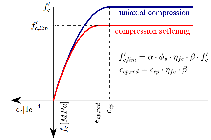
\[ \textsf{\textit{\footnotesize{Fig. 76\qquad The stress-strain diagram of concrete for Strength analysis}}}\]

A CSFM implementációja az IDEA StatiCa Detail-ben nem vesz figyelembe explicit tönkremeneteli kritériumot az alakváltozások tekintetében nyomott beton esetén (azaz a csúcsfeszültség elérése után képlékeny ágat vesz figyelembe ε_c₀ maximális értékkel, legfeljebb 5%-ig, míg az AS 3600 Cl. 8.3.1 szerint az ultimátus alakváltozás kisebb mint 0,3%). Ez az egyszerűsítés nem teszi lehetővé a nyomásban tönkremenő szerkezetek alakváltozási kapacitásának ellenőrzését. A szilárdság azonban megfelelően becsülhető, ha a repedezett beton tényezőjén (k_c₂, amelyet a (77. ábra) definiál) túlmenően a beton ridegségének növekedését – a szilárdság emelkedésével – az \(\eta_{fc}\) redukciós tényező segítségével is figyelembe veszik, amelyet a fib Model Code 2010 az alábbiak szerint definiál:

\[f'_{c,lim}=\alpha_{2}\cdot\phi_{s}\cdot \beta \cdot \eta_{fc}\cdot f'_{c}\]

\[{\eta _{fc}} = {\left( {\frac{{30}}{{{f'_{c}}}}} \right)^{\frac{1}{3}}} \le 1\]

ahol:

α₂ a beton nyomószilárdsági redukciós tényezője, amelyet az AS 3600 Cl. 8.3.1 definiál
Parabola-téglalap feszültség-alakváltozás diagram alkalmazásakor szükséges a maximális nyomófeszültséget ezzel a tényezővel csökkenteni. Ez a nyomási zónában a feszültségeloszlást úgy átlagolja, hogy az eredő nyomószilárdság kisebb vagy egyenlő legyen a csökkenő képlékeny ággal rendelkező feszültség-alakváltozás diagramból számított nyomószilárdsággal. Analóg megközelítés van definiálva a téglalap alakú feszültségtömb esetére a 8.1.3. fejezetben.

Φ_sa beton feszültségredukciós tényezője. Az alapértelmezett érték az AS 3600 2.2.3. táblázata szerint van beállítva.

β a keresztirányú repedezés jelenlétéből adódó redukciós tényező (ebben a szövegben k_c₂-ként is hivatkoznak rá)

f'_c a beton hengerszilárdsága (MPa-ban az \( \eta_{fc} \) definíciójához).

\[ \textsf{\textit{\footnotesize{Fig. 77\qquad The compression softening law.}}}\]

β egy redukciós tényező, amely ugyanazon elveken alapul, mint a 2.2.3. fejezetben definiált effektív nyomószilárdsági tényező. Az e tényező meghatározásához felhasznált irodalom (az AS3600 szabvány kontextusával együtt) megtalálható az AS3600:2018 Sup 1:2022 CL. C2.2.3-ban.

Beton – Használhatóság

A használhatósági vizsgálat a szilárdságszámításhoz alkalmazott anyagmodellek bizonyos egyszerűsítéseit tartalmazza. A beton nyomási feszültség-alakváltozás görbéjének képlékeny ágát figyelmen kívül hagyják, míg a rugalmas ág lineáris és végtelen. A nyomási lágyulás törvényét nem veszik figyelembe. Ezek az egyszerűsítések javítják a numerikus stabilitást és a számítási sebességet, és nem csökkentik a megoldás általánosságát, amennyiben a használhatósági állapotban kapott anyagfeszültségek egyértelműen a folyási határuk alatt maradnak (ahogyan azt az AS3600 megköveteli). Ezért a használhatósági vizsgálathoz alkalmazott egyszerűsített modellek csak akkor érvényesek, ha minden ellenőrzési követelmény teljesül.

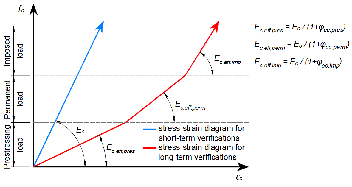
\[ \textsf{\textit{\footnotesize{Fig. 78\qquad Concrete stress-strain diagrams implemented for serviceability analysis: short- and long-term verifications.}}}\]

Hosszú távú hatások

A használhatósági vizsgálatban a beton hosszú távú hatásait az AS 3600 CL 3.1.8 szerinti tervezési kúszási tényező (φ_cc, alapértelmezés szerint 2,5 értékkel) figyelembevételével kezelik, amely a beton szekansi rugalmassági modulusát (E_c) az alábbiak szerint módosítja:

\[E_{c,eff} = \frac{E_{c}}{1+\varphi_{cc}}\]

A teherinkrementumok sorban kerülnek kiszámításra a következő sorrendben: Előfeszítés – Állandó – Változó, az egyes inkrementumokhoz megfelelő effektív rugalmassági modulus alkalmazásával, ahogyan azt a 78. ábra mutatja. A kúszási tényezőket a felhasználó adja meg az anyagtulajdonságokban, és azokat az AS 3600 CL 3.1.8.3 szerint kell meghatározni.

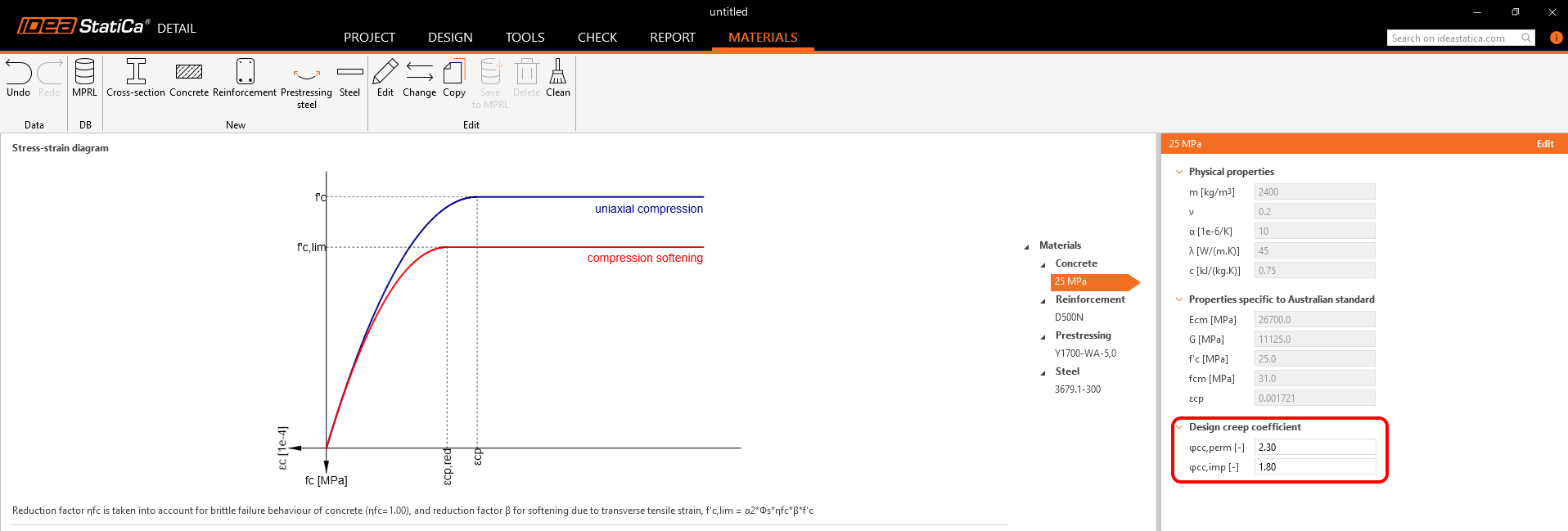
\[ \textsf{\textit{\footnotesize{Fig. 79\qquad Definition of the design creep factor}}}\]

Rövid távú hatások

A rövid távú ellenőrzések elvégzéséhez egy másik számítást végeznek, amelyben az összes terhet az időfüggő tényező nélkül számítják a tartós terhekre. A hosszú és rövid távú ellenőrzések mindkét számítása a 78. ábrán látható.

Vasalás

A nem előfeszített vasaláshoz tökéletesen rugalmas-képlékeny feszültség-alakváltozás diagramot vesznek figyelembe meghatározott folyási ponttal, lásd AS 3600 3.2. szakasz. E diagram meghatározásához csak a vasalás alapvető tulajdonságait kell ismerni – a szilárdságot és a rugalmassági modulust.

A vasalás feszültség-alakváltozás diagramját a felhasználó is megadhatja, de ebben az esetben nem lehet feltételezni a húzási merevítő hatást (nem lehet repedésszélességet számítani).

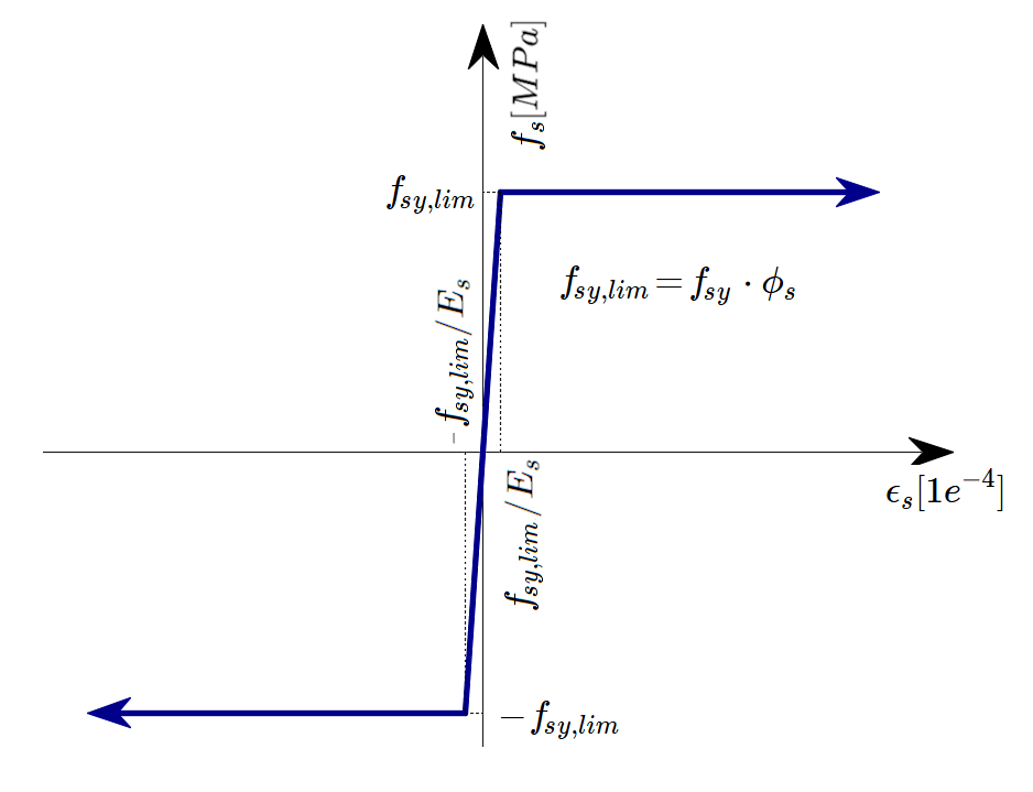
\[ \textsf{\textit{\footnotesize{Fig. 80 \qquad Stress-strain diagram of reinforcement}}}\]

ahol:

Φ_sa vasalás szilárdsági redukciós tényezője. Az alapértelmezett érték az AS 3600 2.2.3. táblázata szerint van beállítva.

f_y a vasalás folyáshatára

E_s a vasalás rugalmassági modulusa

A húzási merevítő hatást (81. ábra) automatikusan veszik figyelembe a szabad vasalórúd bemeneti feszültség-alakváltozás összefüggésének módosításával, hogy megragadják a betonba ágyazott rudak átlagos merevségét (ε_m).

\[ \textsf{\textit{\footnotesize{Fig. 81\qquad Scheme of tension stiffening.}}}\]

7.2 Feszültségcsökkentés és tehertényezők

A feszültségcsökkentő tényezők értékeit az AUS 3600 Cl. 2.2.3 írja elő. A beton és a vasalás alapértelmezett értékei a 2.2.3 táblázat szerint vannak beállítva.

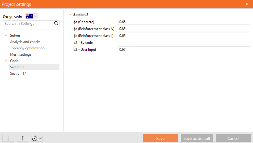
\[ \textsf{\textit{\footnotesize{Fig. 82\qquad The setting of stress reduction factors in IDEA StatiCa Detail.}}}\]

A teherbírási kombinációkhoz tartozó tehertényezőket az AS 3600 Cl. 4.2.2 szerint kell meghatározni. A használhatósági kombinációkhoz tartozó tehertényezőket a 4.1 táblázat szerint kell meghatározni. Minden sablonhoz a tehertényezők már előre meg vannak adva.

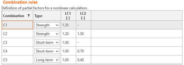
\[ \textsf{\textit{\footnotesize{Fig. 83\qquad The setting of load factors in Idea StatiCa Detail.}}}\]

7.3 Szilárdság és lehorgonyzás ellenőrzések

Az AS 3600 által előírt különböző ellenőrzések a modell által közvetlenül szolgáltatott eredmények alapján kerülnek értékelésre. Az ellenőrzések a beton szilárdságára, a vasalás szilárdságára és a lehorgonyzásra (tapadási nyírófeszültségek) vonatkoznak.

A vasalás szilárdságát húzásban és nyomásban egyaránt a repedéseknél ébredő vasalási feszültség f_s és az előírt határérték f_sy,lim arányaként értékelik.

A tapadási nyírófeszültséget önállóan értékelik, mint a végeselem-analízissel számított tapadási feszültség τ_b és a méretezési végső tapadási feszültség f_bu arányát.

A méretezési végső tapadási feszültség f_bu meghatározásához az alkalmazás az AS3600:2018 Sup 1:2022 szabványban meghatározott C13.1.2.2 képletet veszi figyelembe.

\[f_{bu}=\frac{k_{2}}{k_{1} \cdot k_{3}} \cdot (0.5 \cdot \sqrt{f'_{c}})\]

Ahol f'_c ≤ 65 MPa (a képletben MPa-ban értendő), és a k tényezők az AS 3600 Cl. 13.1.2.2 szerint a következők:

k₃ = 0.7 (konzervatív érték minden vasaláshoz)
k₂ = (132 - d_b) / 100 (d_b a betonacél átmérője milliméterben)
= 1.3 vízszintes betonacélnál, ha a rúd alatt több mint 300 mm beton van betonozva, egyébként 1.0

k₁ automatikusan a modellben lévő vasalás helyzetéből és a betonozás irányából kerül meghatározásra, amely az alkalmazásban minden projektelemhez beállítható az alábbiak szerint.

\[ \textsf{\textit{\footnotesize{Fig. 84\qquad Direction of concreting}}}\]

Az alapvető lehorgonyzási hossz L_sy,tb az AS 3600 13.1.2.2 képlete szerint a következőképpen számítható:

\[L_{sy,tb}=\frac{0.5\cdot k_{1}\cdot k_{3}\cdot f_{sy}\cdot d_{b}}{k_{2}\cdot \sqrt{f'_{c}}}\ge 29 \cdot k_{1}\cdot d_{b}\]

Ahogy a képletből látható, az alapvető lehorgonyzási hossz L_sy,tb alulról korlátozott, ezért a méretezési végső tapadási feszültség f_bu értékét az alkalmazásban ugyanígy korlátozni kell, így a következő érvényes:

\[f_{bu}\le \frac{f_{sy}}{116 \cdot k_{1}} \]

Ahol f_sy MPa-ban értendő.

Az f_bu korlát levezetése a következő:

\[f_{bu}= \frac{f_{sy}\cdot A_{s}}{ \pi \cdot d_{b} \cdot L_{sy,tb}}=\frac{f_{sy}\cdot \pi \cdot d_{b}^{2}}{4 \cdot \pi \cdot d_{b} \cdot 29 \cdot k{1} \cdot d_{b}} =\frac{f_{sy}}{116 \cdot k_{1}} \]

Lehetőség van sima betonacélok modellezésére is. További információ itt található: Sima betonacélok a Detail-ban

Teljes erő F_tot és határerő F_lim

A teljes erő F_tot a végeselem-analízis eredménye, és kétféleképpen definiálható.

\[F_{tot}=A_{s} \cdot f_{s}\]

ahol A_s a betonacél keresztmetszetének területe, f_s pedig a rúdban ébredő feszültség.

Vagy a lehorgonyzási erő F_aés a tapadási erő F_bond összegeként.

\[F_{tot}=F_{a}+F_{bond}\]

ahol F_a a lehorgonyzási rugóban ébredő tényleges erő, F_bond pedig a tapadási erő, amely a tapadási feszültség τ_b integrálásával kapható a betonacél l hossza mentén.

\[F_{bond}=C_{s} \cdot \int_{0}^{l}\tau_{b}\left( x \right)dx\]

C_s a betonacél kerülete.

\[F_{lim}=min\left( F_{lim,bond}+F_{au},F_{u} \right)\]

\[F_{u}=f_{y,lim}\cdot A_{s}\]

\[F_{au}=\beta\cdot f_{y,lim}\cdot A_{s}\]

\[F_{lim,bond}=C_{s}\cdot l \cdot f_{bu}\]

ahol C_s a betonacél kerülete, l pedig a betonacél kezdetétől a vizsgált pontig mért hossz.

\[ \textsf{\textit{\footnotesize{Fig. 85\qquad Definition of the limit force Flim}}}\]

\[F_{lim,2}=F_{lim,1}+F_{lim,add}\]

ahol F_lim,add a szomszédos elemek közötti szög nagyságából számított pótlólagos erő. F_lim,2 mindig kisebb kell legyen, mint F_u.

A CSFM-ben elérhető lehorgonyzási típusok közé tartozik az egyenes rúd (azaz lehorgonyzási végi csökkentés nélkül), a szabványos kampó (Standard cog), a szabványos horog (Standard hook), a tökéletes tapadás és a folytonos rúd. Mindezen típusok, valamint a megfelelő β lehorgonyzási együtthatók a 86. ábrán láthatók a hosszvasalás esetére. Az alkalmazott lehorgonyzási együtthatók értékei az AS 3600 Cl. 13.1.2 alapján kerültek meghatározásra. Megjegyzendő, hogy a CSFM háromféle lehorgonyzási véget különböztet meg: (i) nincs csökkentés a lehorgonyzási hosszban, (ii) 50%-os csökkentés a lehorgonyzási hosszban normalizált lehorgonyzás esetén, és (iii) tökéletes tapadás.

\[ \textsf{\textit{\footnotesize{Fig. 86\qquad Available anchorage types and respective anchorage coefficients for longitudinal reinforcing bars in CSFM:}}}\]

\[ \textsf{\textit{\footnotesize{(a) straight bar; (b) Standard cog; (c) Standard hook; (d) perfect bond; (e) continuous bar}}}\]

A kengyelek lehorgonyzási együtthatója mindig β = 1.0.

Az AS 3600 követelményeinek teljesítése érdekében a számításban lehorgonyzási rugót kell alkalmazni; a lehorgonyzási rugót a β együttható módosítja, ezért a felhasználónak a vasalás kezdeti és végső feltételeinek meghatározásakor az elérhető lehorgonyzási típusok egyikét kell alkalmaznia.

7.4 Használhatósági ellenőrzések

A használhatósági ellenőrzések repedésszélesség és elhajlási határértékek alapján készülnek.

Elhajlás

A kiválasztott kombinációtípustól (hosszú távú vagy rövid távú) függően hosszú távú vagy rövid távú elhajlást értékel a program. A maximálisan megengedhető elhajlási értéket a felhasználónak kell meghatároznia, és azt az AS 3600 Cl. 2.3.2 előírásaival összhangban kell figyelembe venni.

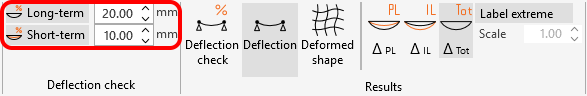
\[ \textsf{\textit{\footnotesize{Fig. 87\qquad Maximum allowable deflection values}}}\]

Az alkalmazásban lehetőség van az állandó terhelésből Δ_PL és a változó terhelésből Δ_IL származó elhajlások külön-külön, valamint a teljes elhajlás Δ_Tot(állandó + változó) megjelenítésére, mindezt az alakváltozott alak megjelenítésével együtt.

A levágott végeken az elhajlások nem ellenőrizhetők.

Repedésszélesség

A repedésszélességek és repedésirányok kiszámítása használhatósági rövid távú vagy hosszú távú kombinációkra történik. A repedésszélesség közvetlen számítási módszere az alkalmazásban az AS 3600 8.6.2.3 szabványban megadott módszeren alapul.

Az ellenőrzések a következőképpen kerülnek bemutatásra:

\[\frac{w}{w_{lim}}\]

ahol:

w a végeselem-módszerrel számított rövid vagy hosszú távú repedésszélesség,

w_lim a felhasználó által meghatározott repedésszélesség határértéke.

Az ajánlott maximális repedésszélességek az AS3600:2018 Sup 1:2022 C2.3.3.1 táblázatában találhatók.

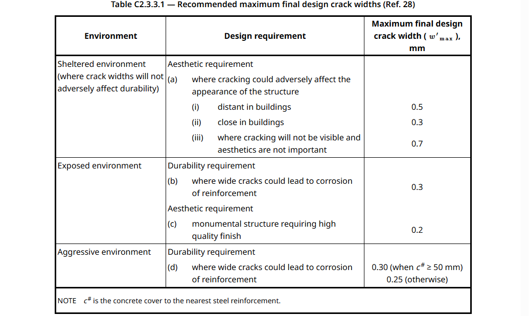
\[ \textsf{\textit{\footnotesize{Fig. 88\qquad Recommended final design crack widths}}}\]

Alternatívaként, az AS3600:2018 Sup 1:2022 Cl. C8.6.1 szerint – A hosszú távú üzemi terhelésnek kitett szerkezetek esetén a w_lim ajánlott értékei a következők:

\[ \textsf{\textit{\footnotesize{Fig. 89\qquad Recommended values for the limit value of the crack width for beams based on exposure classes}}}\]

A repedésszélesség kiszámításának két módja van (stabilizált és nem stabilizált repedezés). Az általános esetben (stabilizált repedezés) a repedésszélességet a vasalórudak 1D elemeinek alakváltozásait integrálva számítják. A repedés iránya ezután az adott vasalási 1D végeselem középpontjához legközelebb eső három integrációs pontból, a 2D betonelem integrációs pontjaiból kerül meghatározásra. Bár ez a repedésirány-számítási megközelítés nem felel meg a repedések valós helyzetének, mégis reprezentatív értékeket ad, amelyek olyan repedésszélesség-eredményekhez vezetnek, amelyek összehasonlíthatók a vasalórud helyzetén a szabvány által előírt repedésszélesség-értékekkel.

8 Előfeszítés – modell leírása

8 Bevezetés és anyagmodellek

A Compatible Stress Field Method (CSFM) egy 2D síkfeszültségen alapuló számítási módszer, amelyben a betont 2D végeselemekkel modellezik, amelyekhez 1D vasalási elemek kapcsolódnak kényszerfeltételek segítségével. A modellhez speciális 1D elemek is hozzáadhatók, amelyek a kötött feszítővasalást képviselik, és amelyek előfeszített, illetve utófeszített módon modellezhetők.

A feszítővasalás modellezése hasonlóan történik a hagyományos vasaláshoz, tengelyirányú erőt átadó lineáris elemek segítségével. Minden egyes feszítővasalás-elem jellemzője a keresztmetszeti területe és anyagtulajdonságai. Ezeket a tulajdonságokat az alkalmazott szabvány (EN 1992-1-1, ACI 318-19 stb.) szerinti jellemző anyaggörbe határozza meg.

EUROCODE

A feszítővasalás feszültség-alakváltozás diagramja: a) Az EN 1992-1-1 szerint meghatározott feszültség-alakváltozás diagram; b) előfeszített vasalás kezdeti alakváltozása

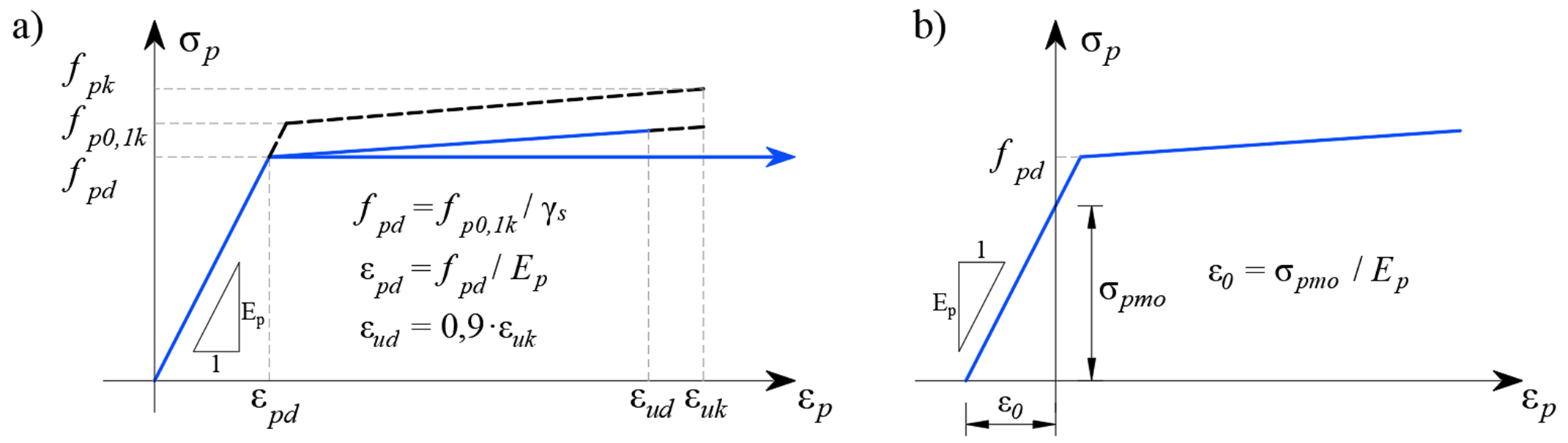
ACI

A feszítővasalás feszültség-alakváltozás diagramja: a) Feszültség-alakváltozás diagram; b) előfeszített vasalás kezdeti alakváltozása

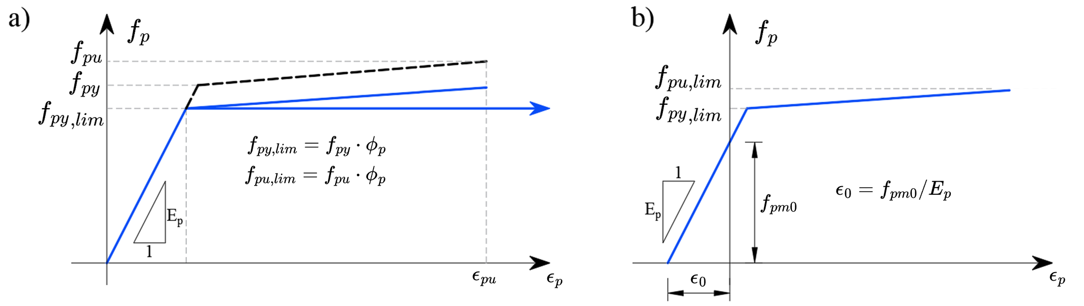
A vasalási elemek tapadási modell segítségével kapcsolódnak a betonmodell 2D elemeihez, ugyanúgy, mint a hagyományos betonvasalás esetén.

Olvassa el: Végeselem-típusok

A tapadási modell elemei lehetővé teszik a feszítővasalás és a beton relatív elmozdulását megfelelő nemlineáris jellemzőkkel. Ez helyesen modellezi a vasalás és a beton kohézióját, valamint az előfeszített vasalás lehorgonyzási modelljét is. Az utófeszített vasalás végi módosításait – pl. a horgonylemez – egy olyan elem modellezi, amelynek merevsége megfelel a feszítővasalás végén lévő horgonynak, a végső feszítőerő pedig területi teherként kerül a betonmodellbe a horgonylemez méretének megfelelő területen. A modell nem képes helyesen leírni a horgony alatti zóna helyi háromtengelyű feszültségállapotát, ezért ezt a zónát külön kell figyelembe venni.

A vasalás húzási merevítő hatása a betonnal való kölcsönhatás miatt nem kerül figyelembevételre a feszítővasalásnál, mivel a feszítővasalás közelében lévő beton nyomott állapotban van.

Előfeszített vasalás

Az előfeszített vasalást az elem betonozása előtt feszítik meg; a feszítővasalás szinte mindig egyenes vonalban halad, ezért súrlódási feszítési veszteség nem lép fel. Miután a szükséges betonszilárdsági értéket elérték, a vasalást felszabadítják a horgonyblokkokból, ezzel aktiválva a feszítővasalást és átadva az erőket a vasalásból a betonba. Ez a hatás fizikailag egyenértékű a vasalás lehűlésével, és a hőterheléshez hasonló kezdeti alakváltozással modellezik. Ennek eredményeként a feszítővasalás feszültség-alakváltozás diagramja a fenti b) ábrán látható módon alakul. A számítási modell automatikusan kiszámítja a szerkezet deformációs válaszát az alkalmazott előfeszítésre, és ezáltal közvetlenül meghatározza az elem rugalmas alakváltozásából eredő feszítési veszteségeket.

Mivel a feszítőerő ismert, és ezért a feszítési feszültség σ_pmo is, a vasalás anyagdiagramja a deformációtól való feszültségfüggéshez használható, és a következőképpen írható fel:

\[{{σ}_{p}}=~{{f}}({{ε}}-{{ε}_{0}})\]

Feltéve, hogy a vasalásban lévő előfeszítés kisebb, mint a folyáshatár (azaz az EN 1992-1-1, 5.10.3 fejezetében meghatározott feltételek teljesülnek), a kezdeti alakváltozás a következőképpen is kiszámítható:

\[{{ε}_{0}}=\frac{{{σ}_{pm0}}}{{{E}_{p}}}\]

ε₀ - előfeszítésből eredő kezdeti alakváltozás
σ_pm0 - feszültség közvetlenül az elengedés előtt
E_p - feszítővasalás rugalmassági modulusa

Az előfeszített vasalás sajátossága, hogy a végek lehorgonyzása több különböző mechanizmus révén valósul meg – a vasalás és a beton molekuláris szintű tapadása, a vasalás felülete és a beton közötti érintkezési felületen keletkező súrlódás, a spirális vasalás mechanikai benyomódása a betonba, valamint a feszítővasalás átmérőjének növekedése, amelyet ék-mechanizmusnak vagy Hoyer-hatásnak neveznek. Az említett hatásokat a CSFM számítási modell az előfeszített vasalás végső zónájában a lehorgonyzási modell tulajdonságainak módosításával veszi figyelembe.

Az előfeszített vasalás és a beton kölcsönhatása: a) spirális vasalás benyomódása a betonba; b) Hoyer-hatás

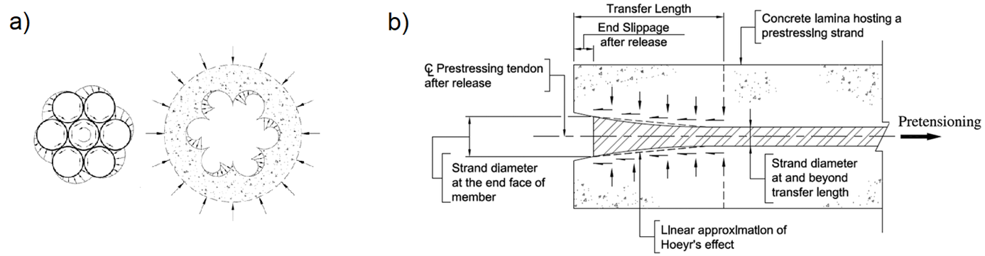
Utófeszített vasalás

Az utófeszített vasalást a szerkezet betonozása után feszítik meg. A feszítőberendezés közvetlenül a szerkezetben támaszkodik, így kiküszöbölve az előfeszítésből eredő rugalmas alakváltozás miatti veszteségeket. Miután a kívánt feszítőerőt elérték, a vasalást lehorgonyozzák, majd a kábelcsatornákat injektálják, ezáltal biztosítva a vasalás és a szerkezet közötti tapadást. Az utófeszített vasalás modellezésekor a számítás ezért több terhelési lépésre oszlik – előfeszítés, egyéb állandó terhek alkalmazása és változó terhek alkalmazása.

Végeselem beton háló csatolt 1D feszítővasalás-elemekkel:

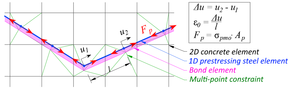
„Előfeszítés" terhelési lépés

A vasalás feszítésekor a vasalás merevsége nem kerül be a szerkezet merevségébe. Ebben a terhelési lépésben a lineáris elem merevsége nem szerepel a modellben; a vasalási elemeket egy helyettesítő teher váltja fel, amely megfelel a feszítési feszültségnek és a vasalás keresztmetszeti területének, ahogy a fenti ábrán látható. Miután a feszítésből eredő teljes terhelést elérték és ez a terhelési lépés konvergált, leolvasásra kerül az adott lineáris elem deformációja, amelynek alapján meghatározzák a feszítővasalás egyes lineáris elemeinek ε₀ kezdeti alakváltozását.

A feszítési feszültség a vasalás hossza mentén manuálisan megadható, vagy automatikusan kiszámítható a vasalás geometriája alapján. Ha az automatikus veszteségszámítást választják, figyelembe veszik a súrlódási veszteséget (az EN 1992-1-1, 5.10.5.2 vagy az ACI 318-19, 20.3.2 szerint) és a lehorgonyzás során bekövetkező vasalás-elcsúszást (horgonykúpok benyomódása). Mivel az összes feszítővasalás egy lépésben kerül alkalmazásra, az egymást követő feszítésből eredő veszteség nem kerül figyelembevételre.

Ezt követő terhelési lépések a feszítővasalás bevonásával

A következő terhelési lépésekben (egyéb állandó és változó terhek alkalmazása) ugyanaz az eljárás követendő, mint az előfeszített vasalás esetén. A feszítővasalás teljes merevsége figyelembe van véve, a vasalás és a körülvevő beton közötti tapadás figyelembe van véve, és a feszítővasalás feszültség-alakváltozás diagramját a ε₀ kezdeti alakváltozással módosítják. Ez az alakváltozás elemenként eltérő, és az előző „előfeszítés" terhelési lépésből nyerhető. A vasalás és a beton közötti tapadás révén a külső terhelésből eredő szerkezeti rugalmas alakváltozás miatti előfeszítés-változás helyesen kerül figyelembevételre a modellben.

Ingyenes próbaverzió indítása

Hivatkozások

ACI Committee 318. 2019. Building Code Requirements for Structural Concrete (ACI 318-19) and Commentary. Farmington Hills, MI: American Concrete Institute.

Alvarez, Manuel. 1998. Einfluss des Verbundverhaltens auf das Verformungsvermögen von Stahlbeton. IBK Bericht 236. Basel: Institut für Baustatik und Konstruktion, ETH Zurich, Birkhäuser Verlag.

Beeby, A. W. 1979. "The Prediction of Crack Widths in Hardened Concrete." The Structural Engineer 57A (1): 9–17.

Broms, Bengt B. 1965. "Crack Width and Crack Spacing In Reinforced Concrete Members." ACI Journal Proceedings 62 (10): 1237–56. https://doi.org/10.14359/7742.

Burns, C.. 2012. "Serviceability Analysis of Reinforced Concrete Members Based on the Tension Chord Model." IBK Report Nr. 342, Zurich, Switzerland: ETH Zurich.

Crisfield, M. A. 1997. Non-Linear Finite Element Analysis of Solids and Structures. Wiley.

European Committee for Standardization (CEN). 2015. 1 Eurocode 2: Design of concrete structures - Part 1-1: General rules and rules for buildings. Brussels: CEN, 2005.

Fernández Ruiz, M., and A. Muttoni. 2007. "On Development of Suitable Stress Fields for Structural Concrete." ACI Structural Journal 104 (4): 495–502.

Kaufmann, W., J. Mata-Falcón, M. Weber, T. Galkovski, D. Thong Tran, J. Kabelac, M. Konecny, J. Navratil, M. Cihal, and P. Komarkova. 2020. "Compatible Stress Field Design Of Structural Concrete. Berlin, Germany."AZ Druck und Datentechnik GmbH, ISBN 978-3-906916-95-8.

Kaufmann, W., and P. Marti. 1998. "Structural Concrete: Cracked Membrane Model." Journal of Structural Engineering 124 (12): 1467–75. https://doi.org/10.1061/(ASCE)0733-9445(1998)124:12(1467).

Kaufmann, W.. 1998. "Strength and Deformations of Structural Concrete Subjected to In-Plane Shear and Normal Forces." Doctoral dissertation, Basel: Institut für Baustatik und Konstruktion, ETH Zürich. https://doi.org/10.1007/978-3-0348-7612-4.

Konečný, M., J. Kabeláč, and J. Navrátil. 2017. Use of Topology Optimization in Concrete Reinforcement Design. 24. Czech Concrete Days (2017). ČBS ČSSI. https://resources.ideastatica.com/Content/06_Detail/Verification/Articles/Topology_optimization_US.pdf.

Marti, P. 1985. "Truss Models in Detailing." Concrete International 7 (12): 66–73.

Marti, P. 2013. Theory of Structures: Fundamentals, Framed Structures, Plates and Shells. First edition. Berlin, Germany: Wiley Ernst & Sohn.

http://sfx.ethz.ch/sfx_locater?sid=ALEPH:EBI01&genre=book&isbn=9783433029916.

Marti, P., M.Alvarez, W. Kaufmann, and V. Sigrist. 1998. "Tension Chord Model for Structural Concrete." Structural Engineering International 8 (4): 287–298.

https://doi.org/10.2749/101686698780488875.

Mata-Falcón, J. 2015. "Serviceability and Ultimate Behaviour of Dapped-End Beams (In Spanish: Estudio Del Comportamiento En Servicio y Rotura de Los Apoyos a Media Madera)." PhD thesis, Valencia: Universitat Politècnica de València.

Meier, H. 1983. "Berücksichtigung Des Wirklichkeitsnahen Werkstoffverhaltens Beim Standsicherheitsnachweis Turmartiger Stahlbetonbauwerke." Institut für Massivbau, Universität Stuttgart.

Navrátil, J., P. Ševčík, L. Michalčík, P. Foltyn, and J. Kabeláč. 2017. A Solution for Walls and Details of Concrete Structures. 24. Czech Concrete Days.

Schlaich, J., K. Schäfer, and M. Jennewein. 1987a. "Toward a Consistent Design of Structural Concrete." PCI Journal 32 (3): 74–150.

Standards Australia. 2018. Concrete Structures (AS 3600:2018). Sydney, NSW: Standards Australia.

Standards Australia. 2022. Concrete Structures – Commentary (Supplement 1 to AS 3600:2018). Sydney, NSW: Standards Australia.

Vecchio, F.J., and M.P. Collins. 1986. "The Modified Compression Field Theory for Reinforced Concrete Elements Subjected to Shear." ACI Journal 83 (2): 219–31.

Kapcsolódó cikkek

Concrete

Tudásbázis

CSFM magyarázata

Detail 2D

EN (Eurocode)

+15

Concrete

Ellenőrzések

Kis kengyel mennyiségű gerendák nyírási vizsgálatai

Detail 2D

Reinforcement

Concrete

Webinárium

Keretcsomópontok – Egy Tipikus D-régió Probléma

25. 02. 2026

Detail 2D

EN (Eurocode)

Concrete

Case study

Donau City Tower 2

12. 05. 2026

Detail 2D

EN (Eurocode)

IDEA StatiCa Detail – Beton szerkezeti megszakítások szerkezeti tervezése

Navigáció

Beton szerkezeti discontinuitások tervezése az IDEA StatiCa Detail-ben

1 Bevezetés a CSFM módszerbe