Introducere 

Pe măsură ce instrumentele de calcul devin tot mai accesibile și mai ușor de utilizat, inclusiv pentru ingineri cu experiență relativ redusă, nevoia de evaluare critică a analizelor computaționale a crescut în mod corespunzător. În domeniul proiectării structurilor metalice, analiza cu elemente finite (FEA) a îmbinărilor structurale reprezintă următorul pas în rapidă avansare. Cu toate acestea, fiabilitatea unor astfel de analize poate fi stabilită doar printr-un proces sistematic de verificare și validare (V&V). Fără o V&V riguroasă, rezultatele elementelor finite nu au credibilitate și nu pot servi drept bază pentru luarea deciziilor inginerești.

Prezentul articol revizitează capitole selectate din Proiectarea îmbinărilor metalice prin metoda elementelor finite bazată pe componente de František Wald et al., recalculate folosind cea mai recentă versiune a software-ului IDEA StatiCa. În plus, mai multe capitole au fost extinse prin exemple suplimentare, consolidând astfel robustețea și acuratețea procesului de verificare. Această contribuție urmărește să întărească fundamentele metodologice ale proiectării îmbinărilor și să ofere o referință mai fiabilă atât pentru cercetarea academică, cât și pentru practica inginerească.

Fundamente teoretice

Descrierea metodei CBFEM se găsește în două documente online separate de fundamente teoretice:

IDEA StatiCa Connection – Proiectarea structurală a îmbinărilor metalice - introducere generală în metoda CBFEM și modelul de analiză din aplicația Connection.
Verificarea componentelor îmbinărilor metalice (EN) - descrierea implementării Eurocodului (EN) privind verificările necesare.
IDEA StatiCa Member – Stabilitatea elementelor - introducere generală în calculul stabilității, flambajului și analizei geometrice neliniare cu imperfecțiuni (GMNIA) din aplicația Member.

Îmbinări sudate 

Sudură de colț în îmbinare prin suprapunere

Descriere

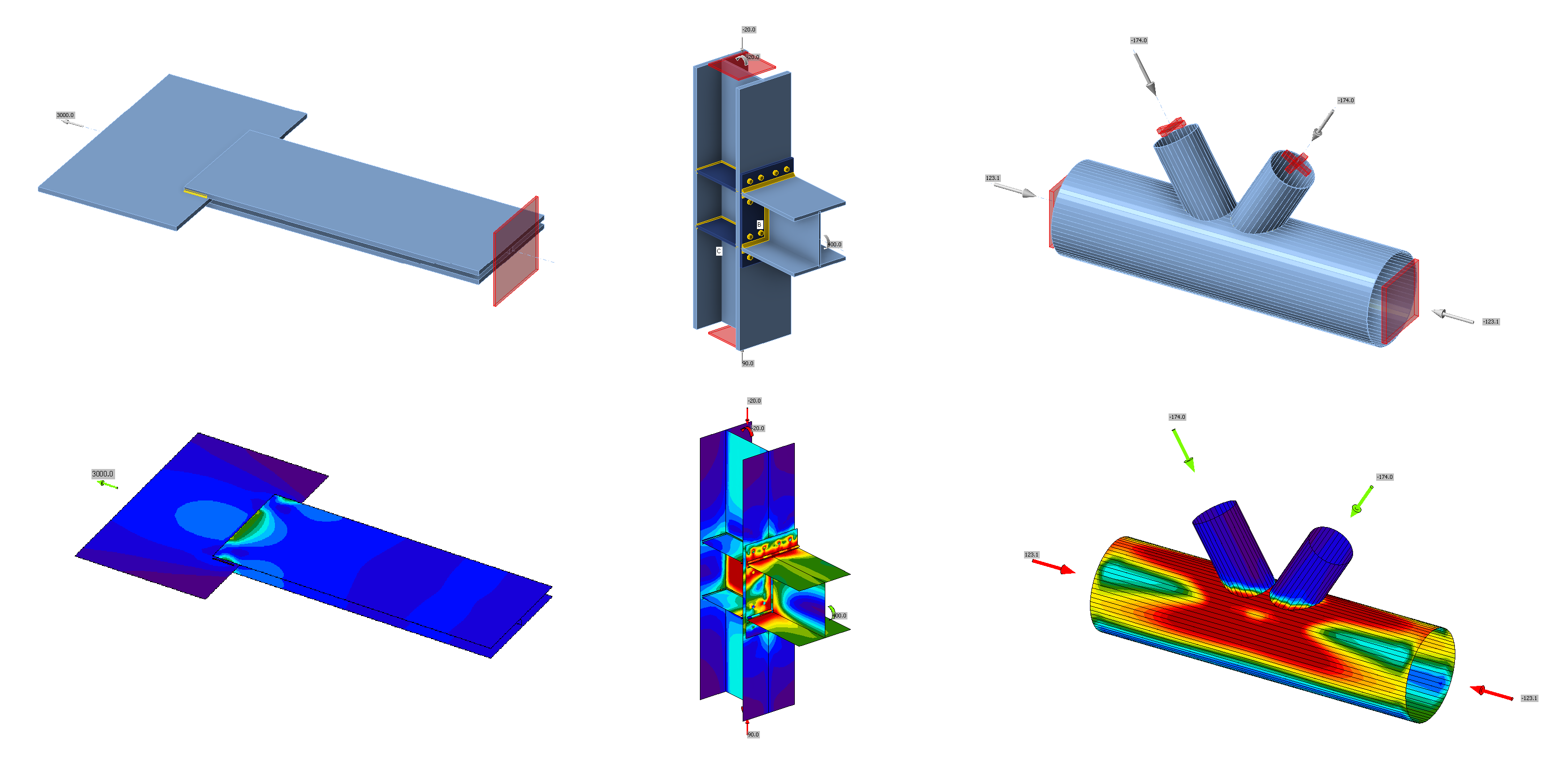
Obiectivul acestui capitol este verificarea metodei elementelor finite bazate pe componente (CBFEM) pentru o sudură de colț într-o îmbinare prin suprapunere, comparativ cu metoda componentelor (CM). Două plăci sunt conectate în trei configurații, și anume cu o sudură transversală, cu o sudură longitudinală și o combinație de suduri transversale și longitudinale. Lungimea și grosimea de calcul a sudurii sunt parametrii variabili în studiu. Studiul acoperă, de asemenea, sudurile lungi a căror rezistență este redusă din cauza concentrării tensiunilor. Îmbinarea este încărcată cu o forță normală.

Model analitic

Sudura de colț este singura componentă examinată în studiu. Sudurile sunt proiectate să fie componenta cea mai slabă din îmbinare. Sudura este proiectată conform EN 1993-1-8:2005. Rezistența de calcul a sudurii de colț este determinată folosind metoda direcțională prezentată în Cl. 4.5.3.2 din EN 1993-1-8:2005. Metodele de calcul disponibile pentru verificarea rezistenței sudurilor de colț se bazează pe ipoteza simplificatoare că tensiunile sunt uniform distribuite în secțiunea de calcul a sudurii de colț, conducând la tensiunile normale și tensiunile tangențiale prezentate în Fig. 4.1.1, după cum urmează:

• σ_⊥ este tensiunea normală perpendiculară pe secțiunea de calcul;
• σ_∥ este tensiunea normală paralelă cu axa sudurii în secțiunea sa transversală;
• τ_⊥ este tensiunea tangențială (în planul secțiunii de calcul) perpendiculară pe axa sudurii;
• τ_∥ este tensiunea tangențială (în planul secțiunii de calcul) paralelă cu axa sudurii.

Tensiunea normală σ_∥ paralelă cu axa nu este luată în considerare la verificarea rezistenței de calcul a unei suduri.

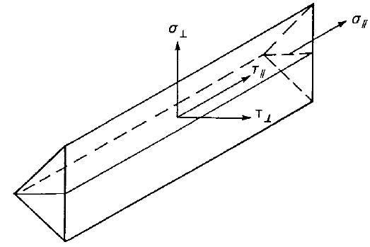
\[ \textsf{\textit{\footnotesize{Fig. 4.1.1 Tensiuni în secțiunea de calcul a unei suduri de colț}}}\]

Rezistența de calcul a sudurii de colț va fi suficientă dacă sunt îndeplinite ambele condiții:

\[ \sqrt{\sigma_{\perp}^2 + 3 \cdot ( \tau_{\perp}^2 + \tau_{\perp}^2 )} \le \frac{f_\textrm{u}}{\beta_\textrm{w} \gamma_\textrm{M2}} \]

\[ \sigma_{\perp} \le \frac{0.9 f_\textrm{u}}{\gamma_\textrm{M2}} \]

În îmbinările prin suprapunere mai lungi de \( 150 \cdot a \), factorul de reducere \(\beta_{\mathrm{Lw,1}}\) este dat de:

\( \beta_{\mathrm{Lw,1}} = 1.2 - \frac{0.2 L_\textrm{j}}{150 a} \)  dar   \(\beta_{\mathrm{Lw,1}} \le 1.0 \)

Model numeric

Componenta de sudură în CBFEM este descrisă în Fundamente teoretice generale și Fundamente teoretice EN. Materialul elastic-plastic neliniar este utilizat pentru suduri în acest studiu. Deformația plastică limită este atinsă în partea mai lungă a sudurii, iar vârfurile de tensiune sunt redistribuite.

Verificarea rezistenței

O prezentare generală a exemplelor considerate și a proprietăților materialelor este furnizată în Tab. 4.1.1. Configurațiile de sudură sunt T pentru transversală, P pentru sudură paralelă și TP pentru o combinație a ambelor; a se vedea geometria în Fig. 4.1.2. Clasa oțelului a fost S235 (f_y = 235 MPa, f_u = 360 MPa, E = 210 GPa, β_w = 0,8). Factorii parțiali de siguranță au fost γ_M0 = 1,0, γ_M2 = 1,25. Geometria modelului este prezentată în Fig. 4.1.2. Plăcile au o grosime de 20 mm. Îmbinarea este simetrică, iar placa este extrasă din îmbinarea sudată. Lungimea și lățimea plăcilor sunt ajustate în funcție de lungimea sudurii paralele și transversale. Rezistența sudurii este întotdeauna modul de cedare determinant. Grosimea de calcul a sudurii este de 3 mm. Lungimile sudurilor transversale și paralele variază în acest studiu parametric.

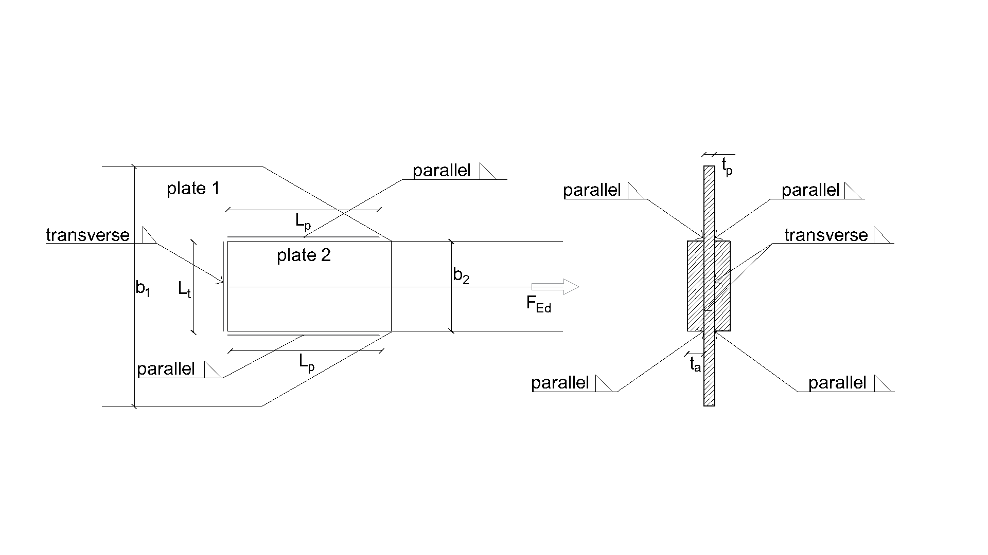
\[ \textsf{\textit{\footnotesize{Desen 4.1 Geometria îmbinării cu dimensiuni}}}\]

Rezistența de calcul a sudurii calculată prin CBFEM este comparată cu rezultatele CM. Rezultatele sunt prezentate în Tab. 4.1.1 – 4.1.3 și Fig. 4.1.3 – 4.1.5.

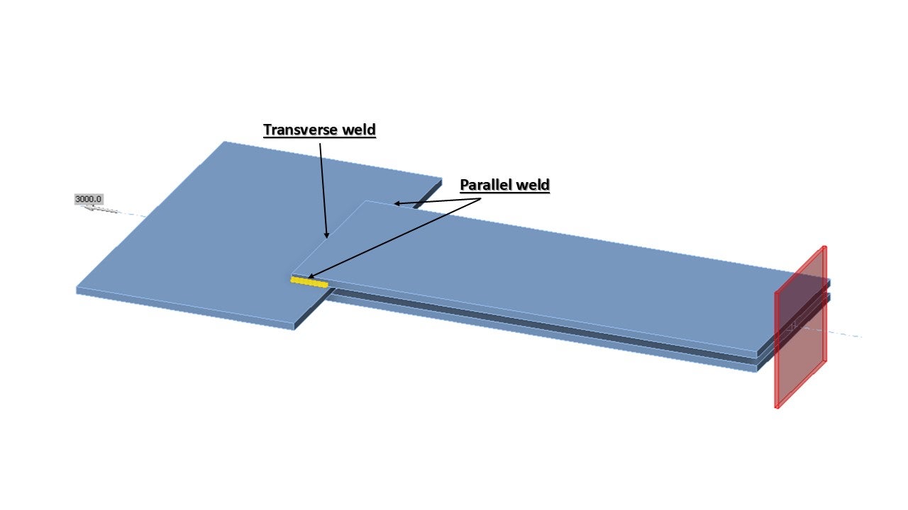
\[ \textsf{\textit{\footnotesize{Fig. 4.1.2 Geometria epruvetei}}}\]

Calculul rezistenței sudurilor transversale 

\[\sqrt{ \sigma_{\perp}^2 + 3 \cdot \left( \tau_{\perp}^2 + \tau_{\parallel}^2\right)} \leq \frac{f_\textrm{u}}{\beta_{\textrm{w}} \cdot \gamma_{\textrm{M2}}}\]

\[\sigma_{\perp} = \tau_{\perp} = \frac{\sigma_\textrm{N}}{\sqrt{2}} = \frac{N}{L_{\textrm{t}} \cdot a}\cdot \frac{1}{\sqrt{2}} \]

\[ \tau_{\parallel} = 0\]

\[ \sqrt{ \left( \frac{\sigma_\textrm{N}}{\sqrt{2}} \right)^2 + 3 \cdot \left( \frac{\sigma_\textrm{N}}{\sqrt{2}} \right)^2} \leq \frac{f_\textrm{u}}{\beta_{\textrm{w}} \cdot \gamma_{\textrm{M2}}}\]

\[ \sqrt{ \left( \frac{N}{L_{\textrm{t}}\cdot a}\cdot \frac{1}{\sqrt{2}} \right)^2 + 3 \cdot \left( \frac{N}{L_{\textrm{t}}\cdot a}\cdot \frac{1}{\sqrt{2}} \right)^2} \leq \frac{f_\textrm{u}}{\beta_{\textrm{w}} \cdot \gamma_{\textrm{M2}}}\]

\[ N \leq \frac{f_\textrm{u} \cdot L_{\textrm{t}}\cdot a }{\beta_{\textrm{w}}  \cdot  \gamma_{\textrm{M2}}  \cdot  \sqrt{2}} \]

\[ \sigma_{\perp}= \frac{N}{L_{\textrm{t}} \cdot a}\cdot \frac{1}{\sqrt{2}} \leq \frac{f_\textrm{u}  \cdot  0.9}{ \gamma_{\textrm{M2}}} \]

\[ N \leq \frac{f_{u}  \cdot L_{\textrm{t}}\cdot  a  \cdot  0.9  \cdot  \sqrt{2}}{ \gamma_{\textrm{M2}} }   \]

Unde:

\(a\) - grosimea de calcul a sudurii

\(N\) - forța normală care acționează asupra elementului

\(L_{\textrm{t}}\) - lungimea totală a sudurii transversale 

\(\beta_{\mathrm{w}}\) - factor de corelație preluat din EN 1993-1-8 Tabelul 4.1

\(f_\textrm{u}\) - rezistența nominală la tracțiune a părții mai slabe îmbinate

\(\gamma_{\mathrm{M2}}\) - factor parțial de siguranță pentru suduri

Calculul rezistenței sudurii paralele

\[\sqrt{ \sigma_{\perp}^2 + 3 \cdot \left( \tau_{\perp}^2 + \tau_{\parallel}^2\right)} \leq \frac{f_\textrm{u}}{\beta_{\mathrm{w}} \cdot \gamma_{\mathrm{M2}}}\]

\[\sigma_{\perp} = \tau_{\perp} = 0 \]

\[ \tau_{\parallel} = \frac{V}{L_{\textrm{p}}  \cdot  a}\]

\[ \sqrt{  3 \cdot \left( \tau_{\parallel} \right)^2} \leq \frac{f_\textrm{u}}{\beta_{\mathrm{w}} \cdot \gamma_{\mathrm{M2}}}\]

\[ \sqrt{  3 \cdot \left(  \frac{V}{L_{\textrm{p}} \cdot a}\right)^2} \leq \frac{f_\textrm{u}}{\beta_{\mathrm{w}} \cdot \gamma_{\mathrm{M2}}}\]

\[ V = \frac{f_\textrm{u}  \cdot  L_{\textrm{p}} \cdot  a  \cdot  \beta_{\mathrm{Lw1}}}{\beta_{\mathrm{w}}  \cdot  \gamma_{\mathrm{M2}}  \cdot  \sqrt{3}} \]

Unde:

\(a\) - grosimea de calcul a sudurii

\(V\) - forța tăietoare care acționează asupra elementului

\(L_{\textrm{t}}\) - lungimea totală a sudurilor paralele

\(\beta_{\mathrm{w}}\) - factor de corelație preluat din EN 1993-1-8 Tabelul 4.1

\(\beta_{\mathrm{Lw1}}\) - factor de reducere pentru suduri lungi, EN 1993-1-8 Ecuația 4.9

\(f_\textrm{u}\) - rezistența nominală la tracțiune a părții mai slabe îmbinate

\(\gamma_{\mathrm{M2}}\) - factor parțial de siguranță pentru suduri

Calculul pentru suduri transversale și paralele 

Rezistența calculată manual pentru o combinație de suduri transversale și paralele este pur și simplu suma rezistențelor transversale și paralele derivate din ecuațiile de mai sus. 

Prezentarea rezultatelor

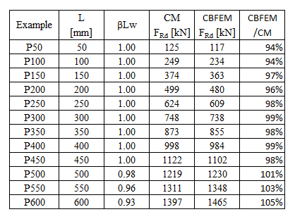
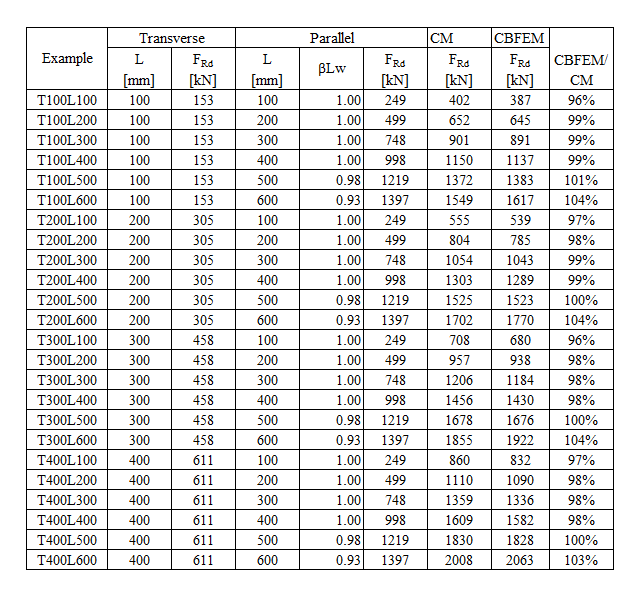
\[ \textsf{\textit{\footnotesize{Tab. 4.1.1 Rezultate suduri paralele}}}\]

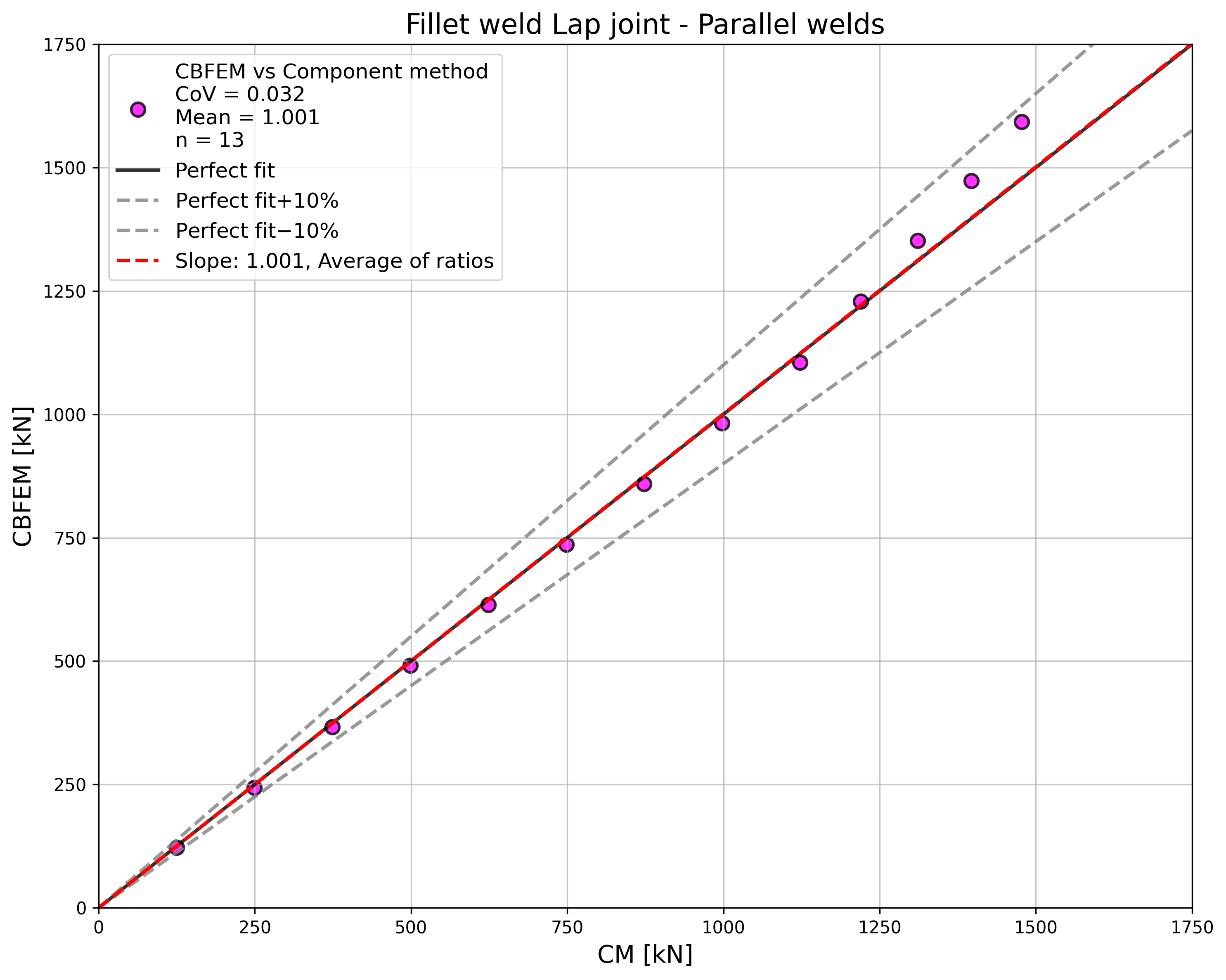
\[ \textsf{\textit{\footnotesize{Fig. 4.1.3 Compararea rezistențelor la încărcare ale sudurilor paralele}}}\]

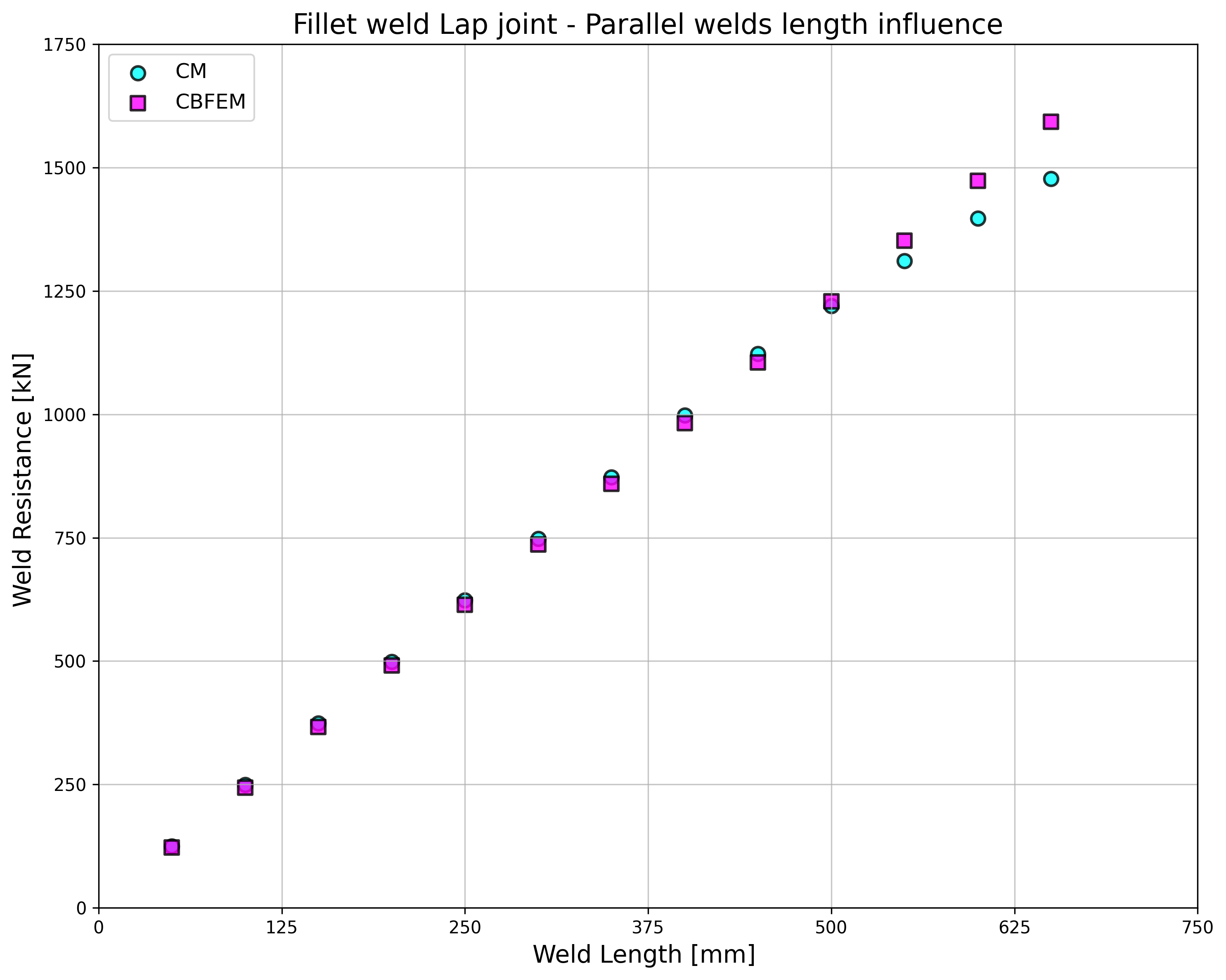
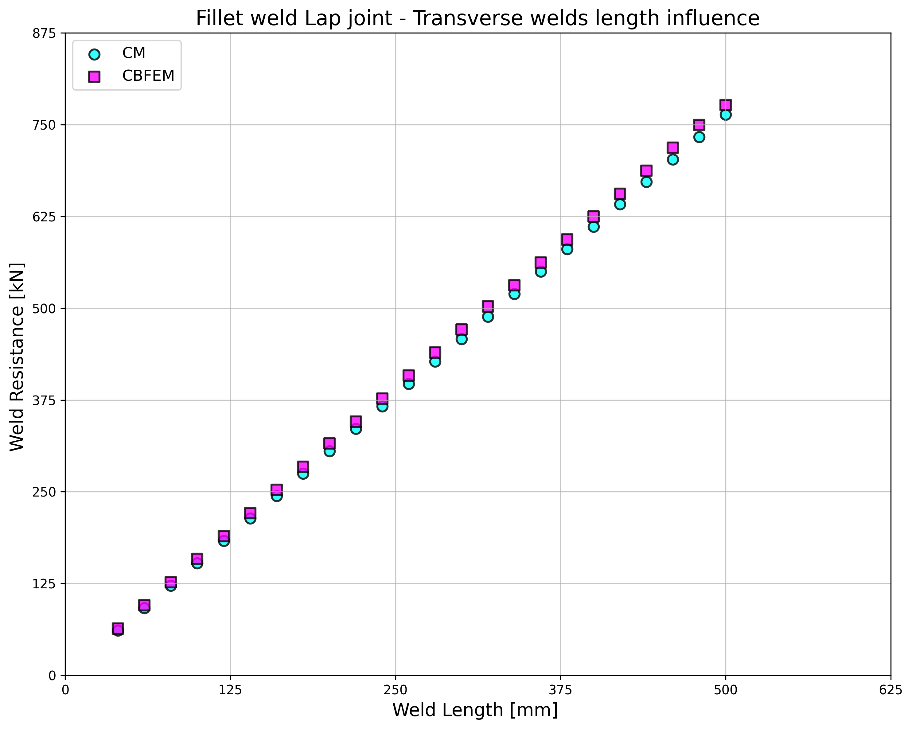
\[ \textsf{\textit{\footnotesize{Fig. 4.1.3.a Influența lungimii sudurii asupra rezistenței}}}\]

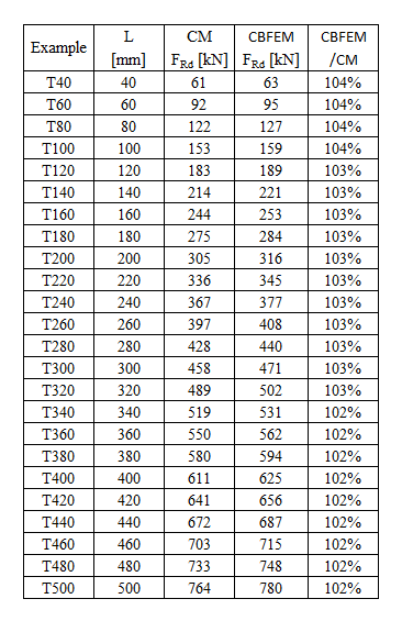
\[ \textsf{\textit{\footnotesize{Tab. 4.1.2 Suduri transversale}}}\]

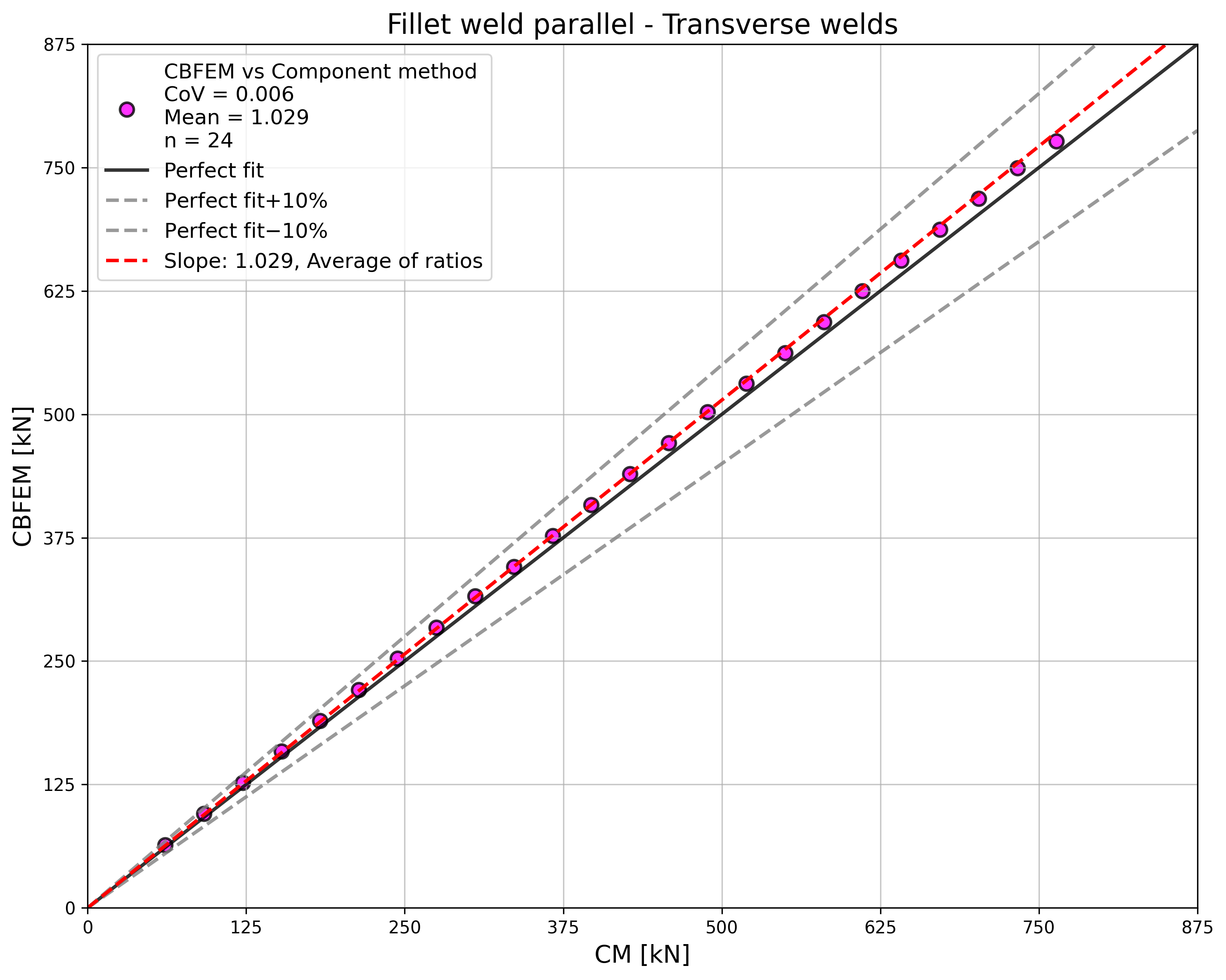
\[ \textsf{\textit{\footnotesize{Fig. 4.1.4 Compararea rezistențelor la încărcare ale sudurilor transversale}}}\]

\[ \textsf{\textit{\footnotesize{Fig. 4.1.4.a Influența lungimii sudurii asupra rezistenței}}}\]

\[ \textsf{\textit{\footnotesize{Tab. 4.1.3 Suduri grupate}}}\]

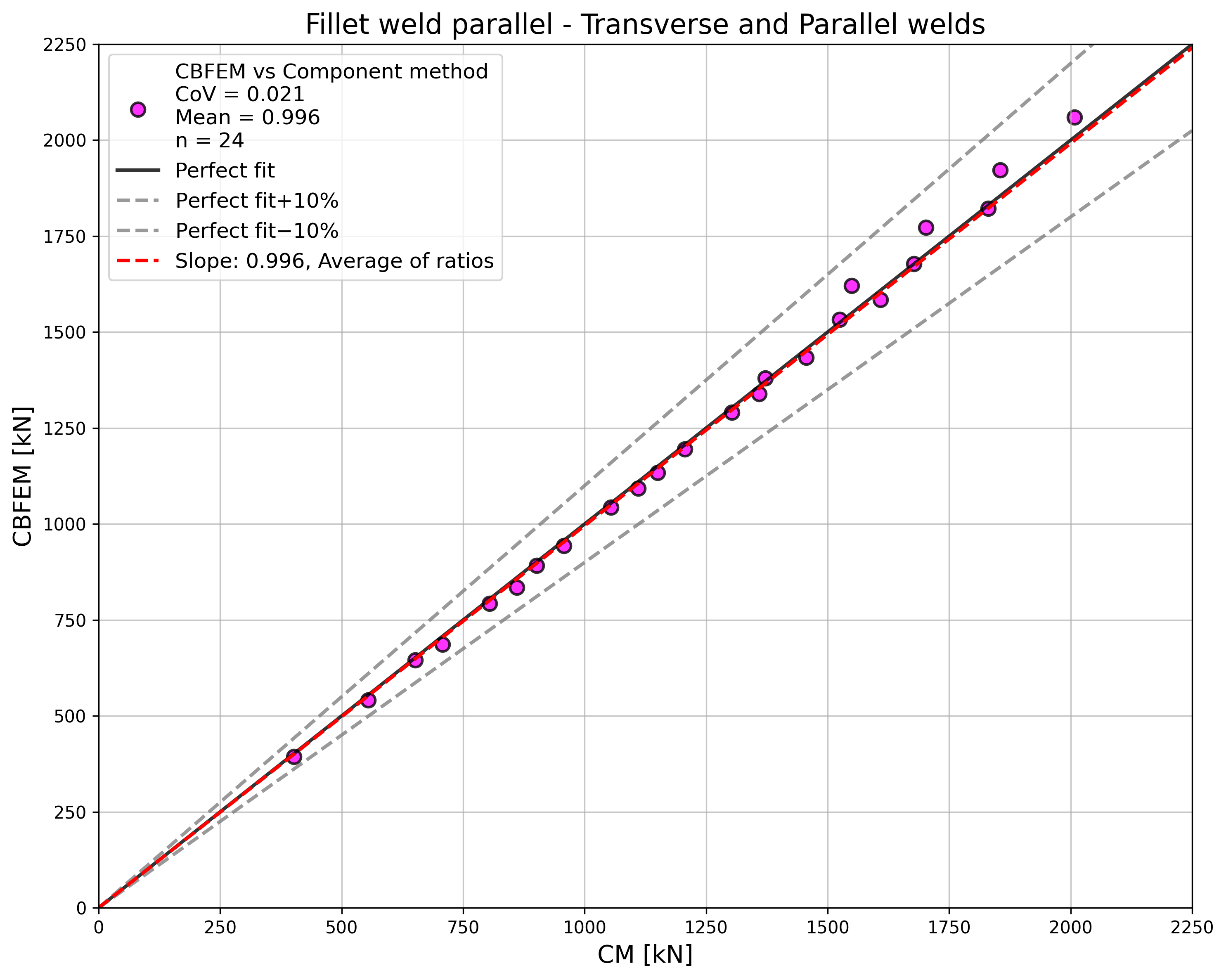
\[ \textsf{\textit{\footnotesize{Fig. 4.1.5 Compararea rezistențelor la încărcare ale grupului}}}\]

Rezistența sudurilor paralele, a sudurilor transversale și a grupurilor de suduri cu orientări multiple este aproape identică conform CM și CBFEM. Cea mai mare diferență din acest studiu este de 6% în rezistența la încărcare.

Rezultatele CBFEM pentru sudurile paralele sunt ușor conservative, dar încep să divergă pentru sudurile lungi. Reducerea rezistenței datorată sudurilor lungi nu este capturată de CBFEM, dar nu se preconizează că suduri mai lungi de 200×grosimea de calcul ar putea apărea în vreo îmbinare, iar până la această lungime, rezultatele sunt în continuare foarte apropiate.

Pentru sudurile transversale, CBFEM furnizează rezultate foarte consistente, cu o rezistență mai mare cu 2–4%.

Exemplu de referință

Date de intrare

Element 1 – Iw60x500

• Sudat din plăci cu grosimea t = 20 mm

• Lățime b = 500 mm

• Inima este eliminată prin operația de fabricație Deschidere

• Oțel S235

Element 2 – Placă 20x1000

• Grosime t = 20 mm

• Lățime b = 1000 mm

• Oțel S235

• Excentricitate e_x = –90 mm

Sudură de colț transversală pe ambele fețe ale Elementului 2

• Grosimea de calcul a = 3 mm

• Lungimea sudurii L_t = 100 mm

Sudură de colț paralelă pe ambele fețe ale Elementului 2

• Grosimea de calcul a = 3 mm

• Lungimea sudurii L_p = 100 mm

Rezultate

• Rezistența de calcul la întindere F_Rd = 387 kN (Trebuie menționat că rezistența a fost calculată folosind funcția „Stop la deformația limită". În consecință, rezistența reală CBFEM poate fi marginal mai mare.)

Sudură de colț în îmbinare cu placă de unghi

Descriere

În acest capitol, modelul sudurii de colț în îmbinarea cu placă de unghi, calculat prin metoda elementelor finite bazată pe componente (CBFEM), este verificat prin metoda componentelor (CM). Un cornier este sudat pe o placă și încărcat cu forță normală. Dimensiunea cornierului și lungimea sudurii sunt studiate într-un studiu de sensibilitate.

Model analitic

Sudura de colț este singura componentă examinată în studiu. Sudurile sunt proiectate conform Capitolului 4 din EN 1993-1-8:2005 pentru a fi cea mai slabă componentă a îmbinării. Rezistența de calcul a sudurii de colț este descrisă în Secțiunea 4.1. Prezentarea generală a exemplelor considerate și a materialului este dată în Tab. 4.2.1. Geometria îmbinărilor cu dimensiuni este prezentată în Fig. 4.2.1.

Calculul prin metoda componentelor 

Acest calcul manual neglijează momentul suplimentar al sudurii, care se dezvoltă datorită redistribuirii forței către părțile secțiunii transversale în L, conform EN 1993-1-8 (4.13).

\[\sqrt{ \sigma_{\perp}^2 + 3 \cdot \left( \tau_{\perp}^2 + \tau_{\parallel}^2\right)} \leq \frac{f_u}{\beta_{\mathrm{w}} \cdot \gamma_{\mathrm{M2}}}\]

\[\sigma_{\perp} = \tau_{\perp} = 0 \]

\[ \tau_{\parallel} = \frac{V}{l  \cdot  a}\]

\[ \sqrt{  3 \cdot \left( \tau_{\parallel} \right)^2} \leq \frac{f_u}{\beta_{\mathrm{w}} \cdot \gamma_{\mathrm{M2}}}\]

\[ \sqrt{  3 \cdot \left(  \frac{V}{l \cdot a}\right)^2} \leq \frac{f_u}{\beta_{\mathrm{w}} \cdot \gamma_{\mathrm{M2}}}\]

\[ V = \frac{f_u  \cdot  l \cdot  a  \cdot  \beta_{\mathrm{Lw1}}}{\beta_{\mathrm{w}}  \cdot  \gamma_{\mathrm{M2}}  \cdot  \sqrt{3}} \]

Rezistența totală calculată ca sumă a rezistențelor sudurii superioare și inferioare 

\[ V = V_\mathrm{top} + V_\mathrm{bottom} \]

Unde:

\(a\) - grosimea gâtului sudurii

\(V\) - forța de forfecare care acționează pe grindă

\(l = 2 \cdot L_\mathrm{\dots}\) - lungimea sudurilor paralele

\(\beta_{\mathrm{w}}\) - factor de corelație preluat din EN 1993-1-8 Tabelul 4.1

\(\beta_{\mathrm{Lw1}}\) - factor de reducere pentru suduri lungi, EN 1993-1-8 Ecuația 4.9

\(f_u\) - rezistența nominală la tracțiune a celei mai slabe piese îmbinate

\(\gamma_{\mathrm{M2}}\) - factor parțial de siguranță pentru suduri

\[ \textsf{\textit{\footnotesize{Tab. 4.2.1 Prezentarea generală a exemplelor}}}\]

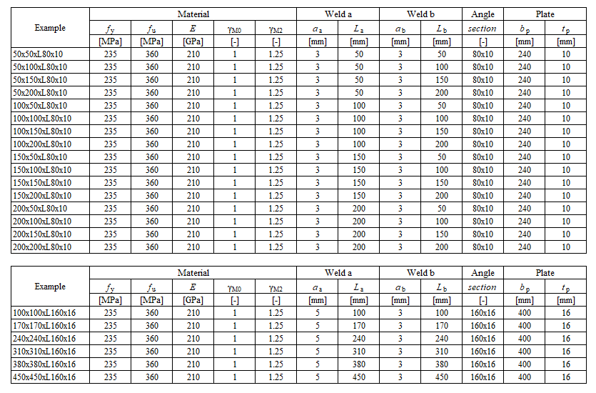
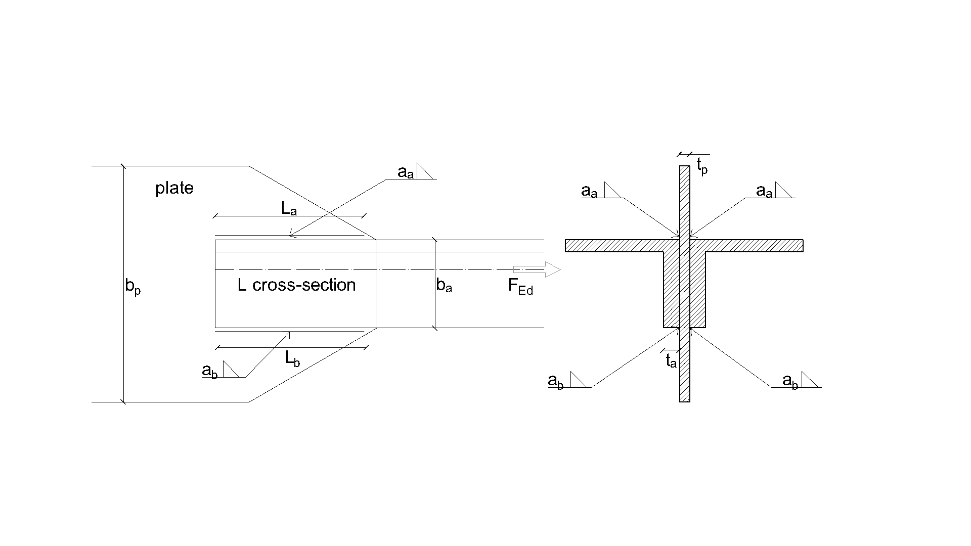
\[ \textsf{\textit{\footnotesize{Fig. 4.2.1 Geometria îmbinării cu dimensiuni}}}\]

Model numeric

Componenta de sudură în CBFEM este descrisă în Fundamente teoretice generale și Fundamente teoretice EN. Modelul de sudură are o diagramă de material elastic-plastică, iar vârfurile de tensiune sunt redistribuite de-a lungul lungimii sudurii.

Verificarea rezistenței

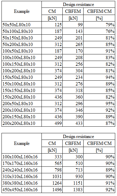
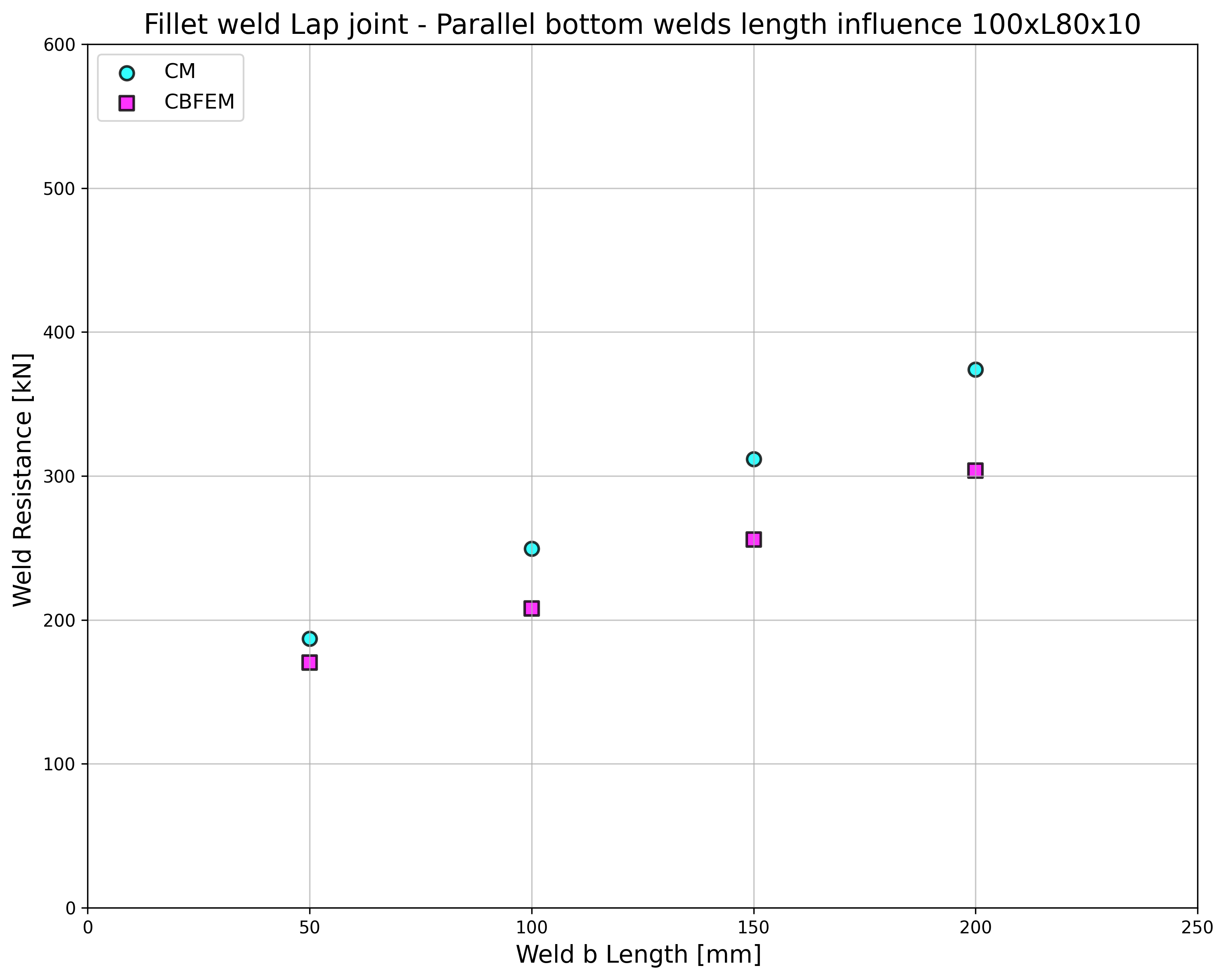
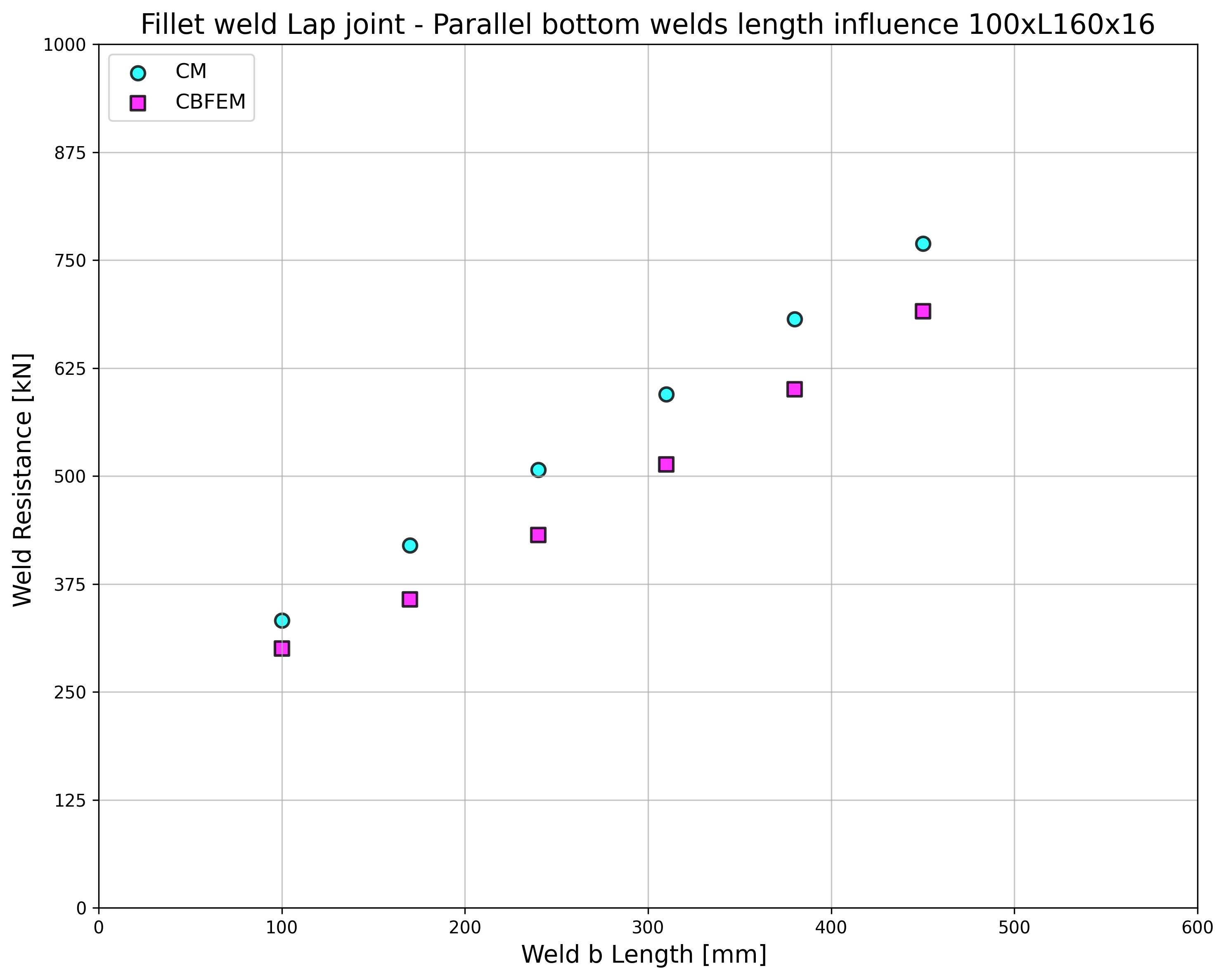
Rezistențele de calcul ale sudurilor calculate prin CBFEM sunt comparate cu rezultatele CM; a se vedea Tab. 4.2.2. Sunt studiați doi parametri: lungimea sudurii și secțiunea cornierului. Fig. 4.2.2 prezintă studiul de sensibilitate al lungimii sudurii inferioare. Lungimea sudurii superioare a în studiu este L_a=100mm.

 \[ \textsf{\textit{\footnotesize{Tab. 4.2.2 Comparație între CBFEM și CM}}}\]

\[ \textsf{\textit{\footnotesize{a}}}\]

\[ \textsf{\textit{\footnotesize{b}}}\]

\[ \textsf{\textit{\footnotesize{a) Cornier de prindere 80×10             b) Cornier de prindere 160×16}}}\]

 \[ \textsf{\textit{\footnotesize{Fig. 4.2.2 Studiu de sensibilitate al lungimii sudurii inferioare b}}}\]

Rezultatele CBFEM și CM sunt comparate, iar studiul de sensibilitate este prezentat. Influența lungimii sudurii asupra rezistenței de calcul a unei îmbinări cu cornier sudat este prezentată în Fig. 4.2.2. Studiul arată o bună concordanță pentru toate configurațiile de sudură. Pentru a ilustra acuratețea modelului CBFEM, rezultatele studiului sunt rezumate într-o diagramă care compară rezistențele de calcul prin CBFEM și CM; a se vedea Fig. 4.2.3. Rezultatele arată că toate predicțiile CBFEM sunt pe partea sigură față de CM, unde excentricitatea este neglijată.

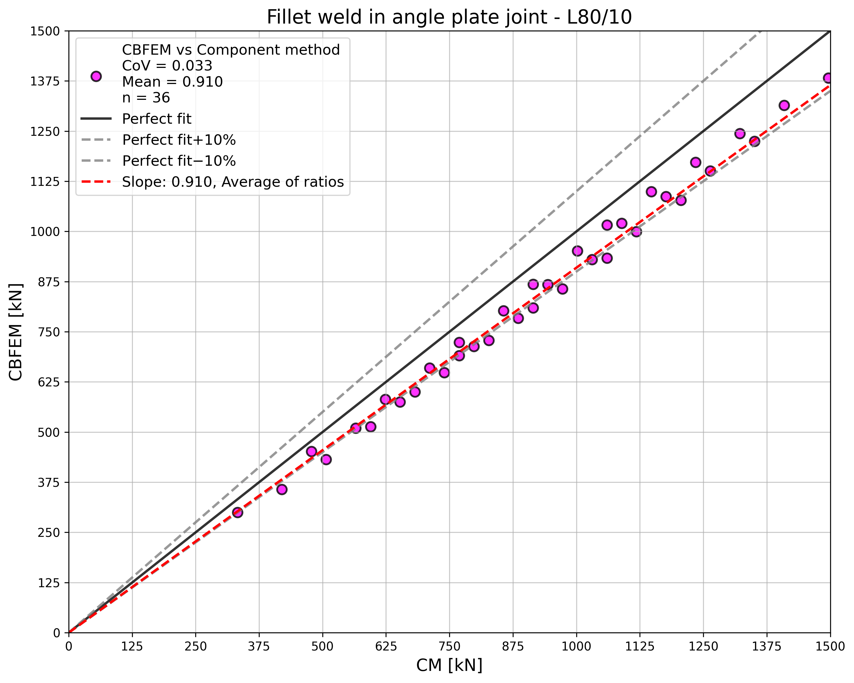
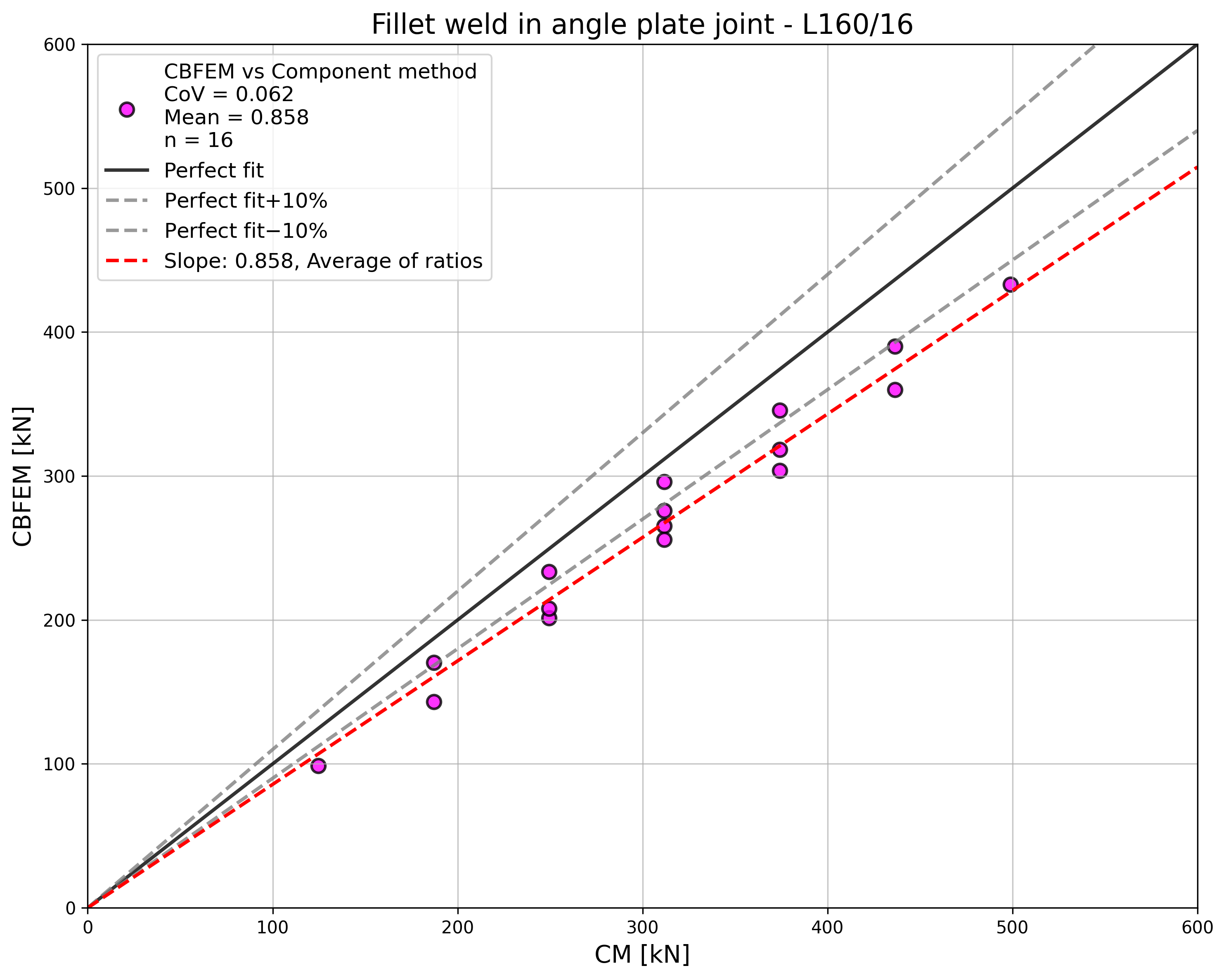
\[ \textsf{\textit{\footnotesize{Fig. 4.2.3 Verificarea CBFEM față de CM}}}\]

Exemplu de referință

Date de intrare

Cornier

• Secțiune transversală 2×L80×10
• Distanța dintre corniere 16 mm

Placă

• Grosime t_p = 16 mm
• Lățime b_p  = 240 mm

Sudură, suduri de colț paralele, a se vedea Fig. 4.2.4

• Grosimea gâtului a_w  = 3 mm
• Lungimea sudurii superioare L_w,top = 100 mm
• Lungimea sudurii inferioare L_w,bottom = 50 mm

Rezultate

• Rezistența de calcul la întindere F_Rd = 170 kN (De remarcat că rezistența a fost calculată utilizând funcția „Stop la deformația limită". În consecință, rezistența reală CBFEM poate fi marginal mai mare.)

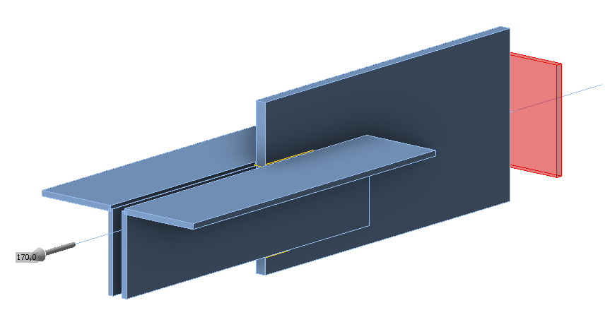
\[ \textsf{\textit{\footnotesize{Fig. 4.2.4 Exemplu de referință al îmbinării cu placă de unghi sudat cu suduri de colț paralele}}}\]

Sudură de colț în îmbinarea cu placă de inimă

Descriere

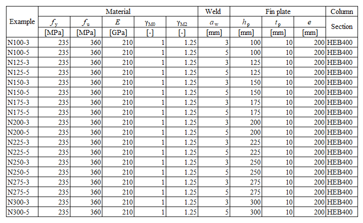
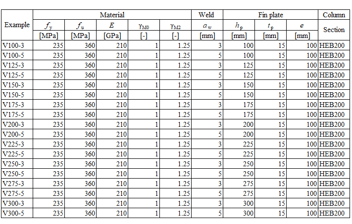
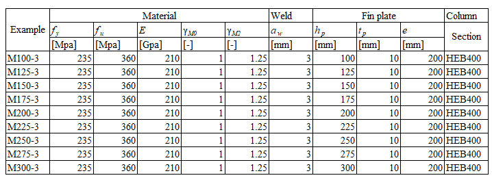
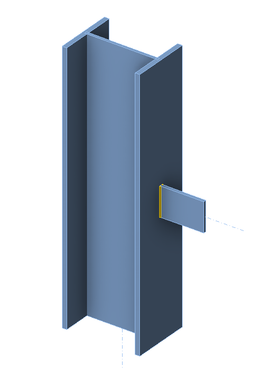
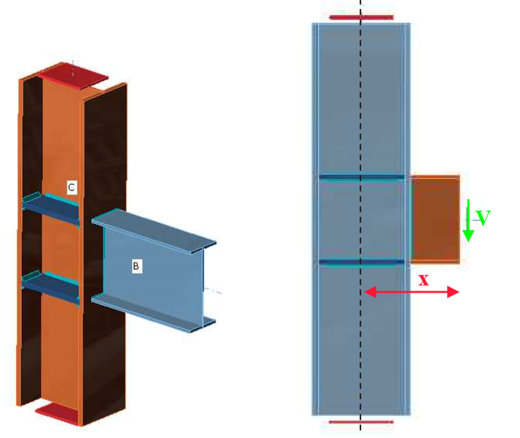
În acest capitol, metoda elementelor finite bazată pe componente (CBFEM) pentru o sudură de colț într-o îmbinare cu placă de inimă este verificată prin metoda componentelor (CM). Placa de inimă este sudată la un stâlp cu secțiune deschisă HEB. Înălțimea plăcii de inimă variază de la 150 la 300 mm. Placa/sudura este încărcată cu forță normală, forță tăietoare și moment încovoietor.

Model analitic

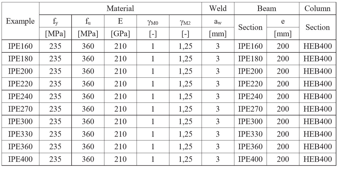
Sudura de colț este singura componentă examinată în studiu. Sudurile sunt proiectate să fie componenta cea mai slabă a îmbinării, conform Capitolului 4 din EN 1993-1-8:2005. Rezistența de calcul a sudurii de colț este descrisă în Secțiunea 4.1. Prezentarea generală a exemplelor considerate și a materialului este dată în Tab. 4.3.1. Sunt considerate trei cazuri de încărcare: forță normală N, forță tăietoare V și moment încovoietor M. Geometria îmbinării cu dimensiunile este prezentată în Fig. 4.3.1.

Calculul rezistenței sudurii la forță normală 

\[\sqrt{ \sigma_{\perp}^2 + 3 \cdot \left( \tau_{\perp}^2 + \tau_{\parallel}^2\right)} \leq \frac{f_u}{\beta_{\mathrm{w}} \cdot \gamma_{\mathrm{M2}}}\]

\[\sigma_{\perp} = \tau_{\perp} = \frac{\sigma_{N}}{\sqrt{2}} = \frac{N}{l \cdot a}\cdot \frac{1}{\sqrt{2}} \]

\[ \tau_{\parallel} = 0\]

\[ \sqrt{ \left( \frac{\sigma_{N}}{\sqrt{2}} \right)^2 + 3 \cdot \left( \frac{\sigma_{N}}{\sqrt{2}} \right)^2} \leq \frac{f_u}{\beta_{\mathrm{w}} \cdot \gamma_{\mathrm{M2}}}\]

\[ \sqrt{ \left( \frac{N}{l \cdot a}\cdot \frac{1}{\sqrt{2}} \right)^2 + 3 \cdot \left( \frac{N}{l_\mathrm{tw} \cdot a}\cdot \frac{1}{\sqrt{2}} \right)^2} \leq \frac{f_u}{\beta_{\mathrm{w}} \cdot \gamma_{\mathrm{M2}}}\]

\[ N \leq \frac{f_{u} \cdot l\cdot a }{\beta_{\mathrm{w}}  \cdot  \gamma_{\mathrm{M2}}  \cdot  \sqrt{2}} \]

\[ \sigma_{\perp} \leq \frac{f_{u}  \cdot  0.9}{ \gamma_{\mathrm{M2}}} \]

\[ N \leq \frac{f_{u}  \cdot  l  \cdot  a  \cdot  0.9  \cdot  \sqrt{2}}{ \gamma_{\mathrm{M2}} }   \]

Unde:

\(a\) - grosimea gâtului sudurii

\(N\) - forța normală care acționează asupra grinzii

\(l\) - lungimea totală a sudurii 

\(\beta_{\mathrm{w}}\) - factor de corelație preluat din EN 1993-1-8 Tabelul 4.1

\(f_u\) - rezistența nominală la tracțiune a elementului mai slab îmbinat

\(\gamma_{\mathrm{M2}}\) - factor parțial de siguranță pentru suduri

Calculul rezistenței sudurii la moment încovoietor 

\[\sqrt{ \sigma_{\perp}^2 + 3 \cdot \left( \tau_{\perp}^2 + \tau_{\parallel}^2\right)} \leq \frac{f_u}{\beta_{\mathrm{w}} \cdot \gamma_{\mathrm{M2}}}\]

\[\sigma_{\perp} = \tau_{\perp} = \frac{\sigma_{N}}{\sqrt{2}} = \frac{M}{W}\cdot \frac{1}{\sqrt{2}} \]

\[ \tau_{\parallel} = 0\]

\[ \sqrt{ \left( \frac{\sigma_{N}}{\sqrt{2}} \right)^2 + 3 \cdot \left( \frac{\sigma_{N}}{\sqrt{2}} \right)^2} \leq \frac{f_u}{\beta_{\mathrm{w}} \cdot \gamma_{\mathrm{M2}}}\]

\[ \sqrt{ \left( \frac{M}{W}\cdot \frac{1}{\sqrt{2}} \right)^2 + 3 \cdot \left( \frac{M}{W}\cdot \frac{1}{\sqrt{2}} \right)^2} \leq \frac{f_u}{\beta_{\mathrm{w}} \cdot \gamma_{\mathrm{M2}}}\]

\[ M \leq \frac{f_{u} \cdot W }{\beta_{\mathrm{w}}  \cdot  \gamma_{\mathrm{M2}}  \cdot  \sqrt{2}} \]

\[ \sigma_{\perp} \leq \frac{f_{u}  \cdot  0.9}{ \gamma_{\mathrm{M2}}} \]

\[ M \leq \frac{f_{u}  \cdot  W  \cdot  0.9  \cdot  \sqrt{2}}{ \gamma_{\mathrm{M2}} }   \]

Unde:

\(a\) - grosimea gâtului sudurii

\(W = \frac{1}{4} \cdot a \cdot l^2\) - modulul de rezistență plastic al sudurii

\(M\) - momentul încovoietor care acționează asupra grinzii

\(l\) - lungimea totală a sudurii 

\(\beta_{\mathrm{w}}\) - factor de corelație preluat din EN 1993-1-8 Tabelul 4.1

\(f_u\) - rezistența nominală la tracțiune a elementului mai slab îmbinat

\(\gamma_{\mathrm{M2}}\) - factor parțial de siguranță pentru suduri

Calculul rezistenței sudurii la forță tăietoare

\[\sqrt{ \sigma_{\perp}^2 + 3 \cdot \left( \tau_{\perp}^2 + \tau_{\parallel}^2\right)} \leq \frac{f_u}{\beta_{\mathrm{w}} \cdot \gamma_{\mathrm{M2}}}\]

\[\sigma_{\perp} = \tau_{\perp} = 0 \]

\[ \tau_{\parallel} = \frac{V}{l \cdot  a}\]

\[ \sqrt{  3 \cdot \left( \tau_{\parallel} \right)^2} \leq \frac{f_u}{\beta_{\mathrm{w}} \cdot \gamma_{\mathrm{M2}}}\]

\[ \sqrt{  3 \cdot \left(  \frac{V}{l \cdot a}\right)^2} \leq \frac{f_u}{\beta_{\mathrm{w}} \cdot \gamma_{\mathrm{M2}}}\]

\[ V = \frac{f_u  \cdot  l\cdot  a  }{\beta_{\mathrm{w}}  \cdot  \gamma_{\mathrm{M2}}  \cdot  \sqrt{3}} \]

Unde:

\(a\) - grosimea gâtului sudurii

\(V\) - forța tăietoare care acționează asupra grinzii

\(l\) - lungimea totală a sudurii

\(\beta_{\mathrm{w}}\) - factor de corelație preluat din EN 1993-1-8 Tabelul 4.1

\(f_u\) - rezistența nominală la tracțiune a elementului mai slab îmbinat

\(\gamma_{\mathrm{M2}}\) - factor parțial de siguranță pentru suduri

\[ \textsf{\textit{\footnotesize{Tab. 4.3.1.N Examples overview}}}\]

\[ \textsf{\textit{\footnotesize{Tab. 4.3.1.V Examples overview}}}\]

\[ \textsf{\textit{\footnotesize{Tab. 4.3.1.M Examples overview}}}\]

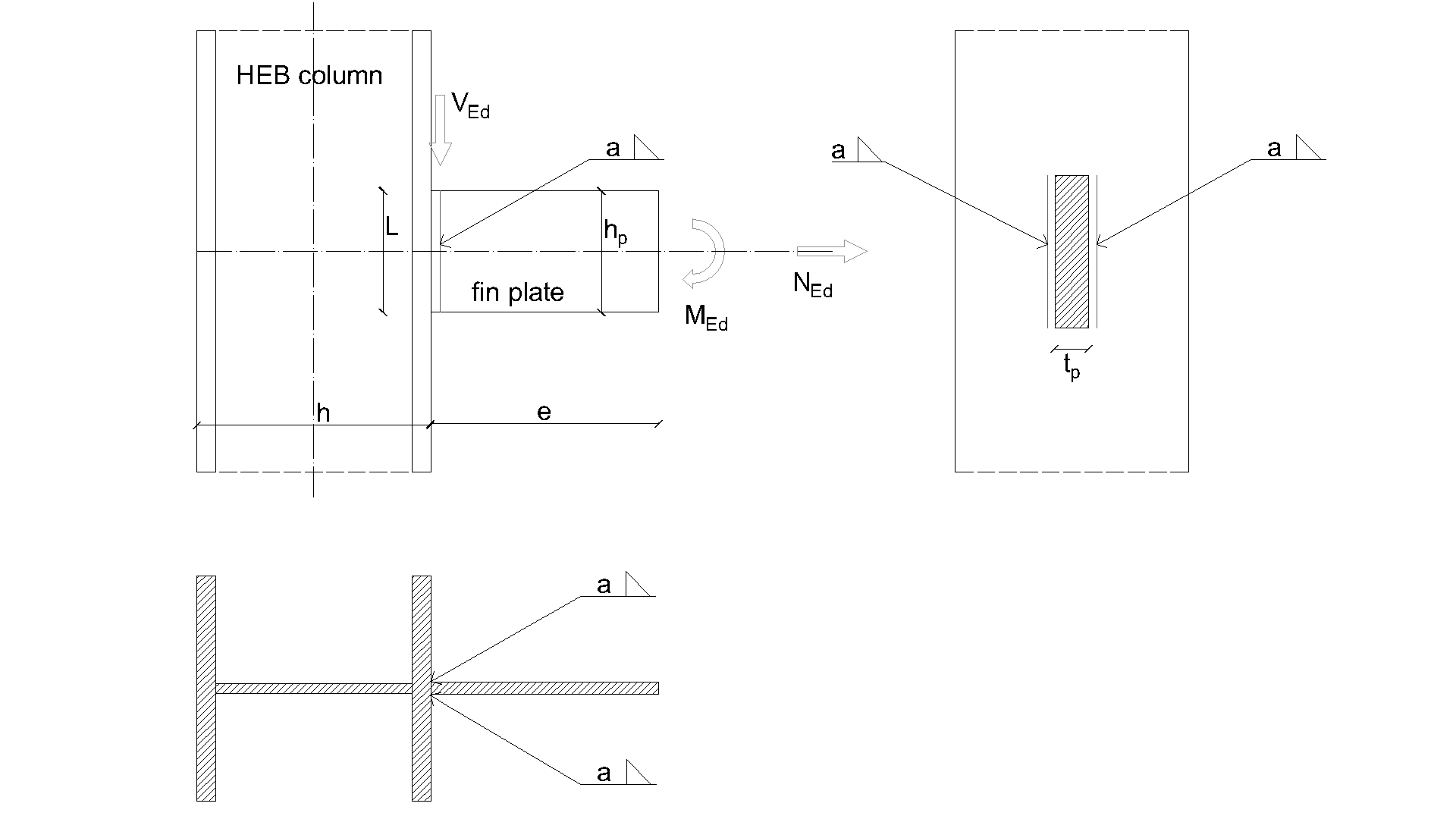
\[ \textsf{\textit{\footnotesize{Fig. 4.3.1 Joint geometry with dimensions}}}\]

Model numeric

Componenta de sudură în CBFEM este descrisă în Fundamente teoretice generale și Fundamente teoretice EN. Modelul de sudură are un diagram elastic-plastic al materialului, iar vârfurile de tensiune sunt redistribuite de-a lungul lungimii sudurii.

Verificarea rezistenței

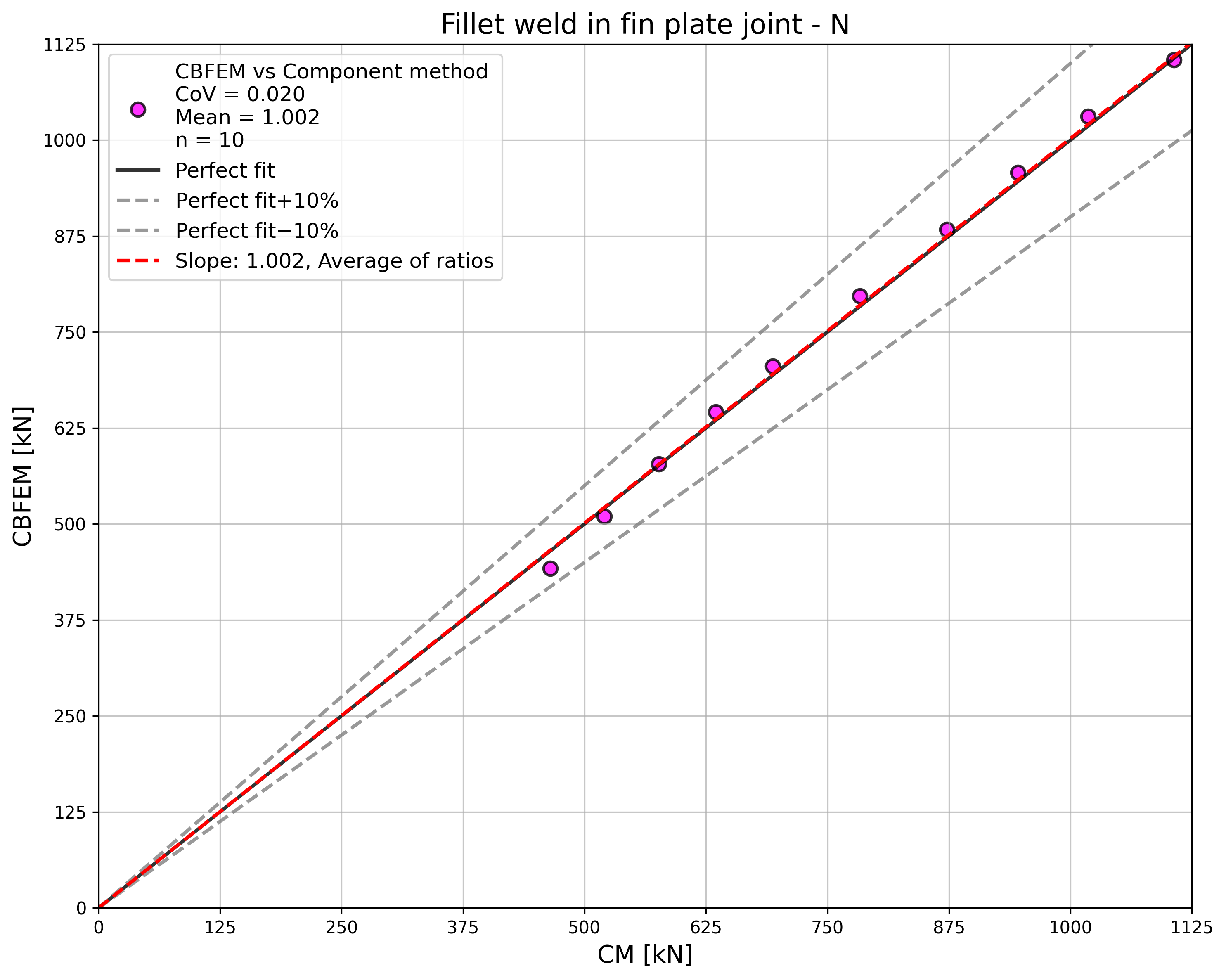
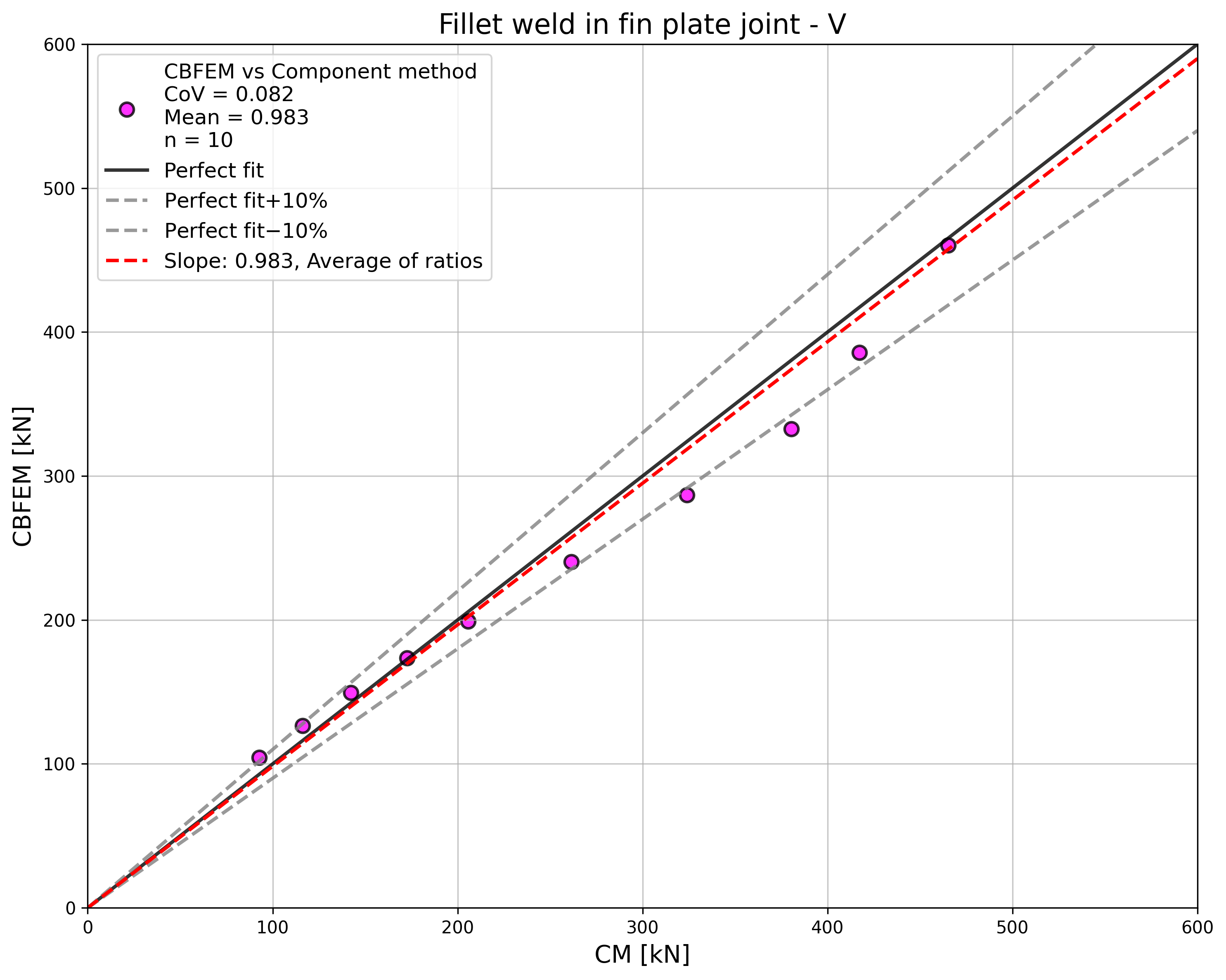
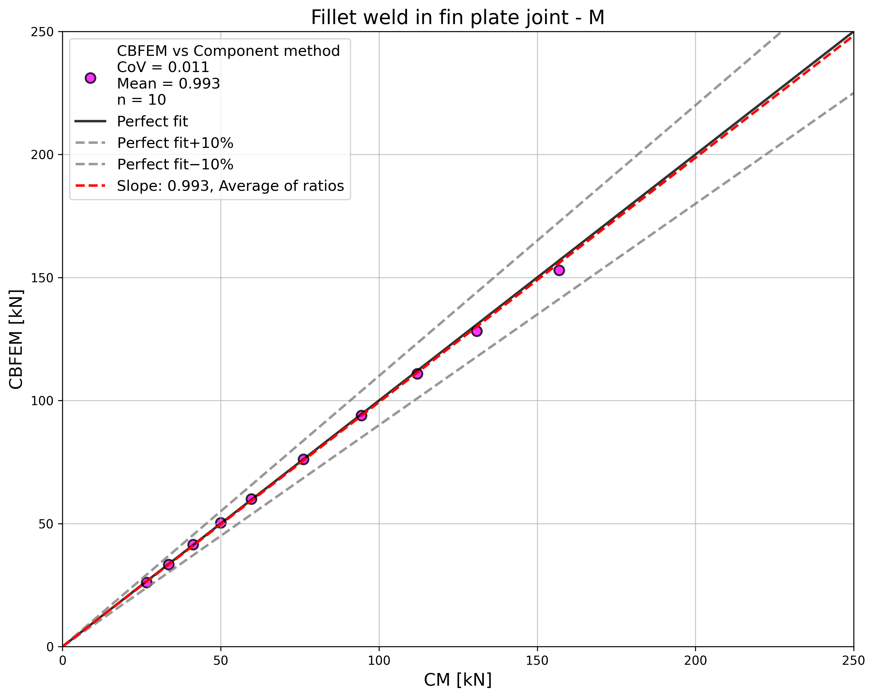
Rezistența de calcul calculată prin CBFEM este comparată cu rezultatele CM. Comparația este prezentată în Tab. 4.3.2. Studiul este realizat pentru un parametru: lungimea sudurii, adică înălțimea plăcii de inimă, și trei cazuri de încărcare: forță normală, forță tăietoare și moment încovoietor. Forța tăietoare este aplicată în planul sudurii pentru a neglija efectul unui moment încovoietor suplimentar. Momentul încovoietor este aplicat la capătul plăcii de inimă. Influența lungimii sudurii asupra rezistenței de calcul a îmbinărilor cu placă de inimă încărcate cu forță normală și forță tăietoare este prezentată în Fig. 4.3.2. Relația dintre lungimea sudurii și rezistența la moment încovoietor a îmbinării este prezentată în Fig. 4.3.3.

\[ \textsf{\textit{\footnotesize{Tab. 4.3.2 Comparison of CBFEM and CM}}}\]

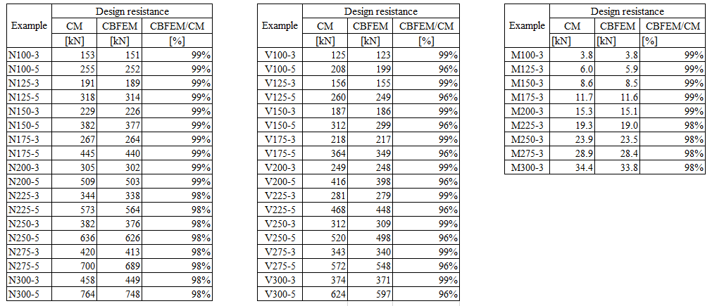
Rezultatele CBFEM și CM sunt comparate, iar studiul de sensibilitate este prezentat. Influența lungimii sudurii asupra rezistenței de calcul într-o îmbinare cu placă de inimă încărcată cu forță normală este prezentată în Fig. 4.3.2, cu forță tăietoare în Fig. 4.3.3 și cu moment încovoietor în Fig. 4.3.4. Studiul arată o concordanță bună pentru toate cazurile de încărcare aplicate.

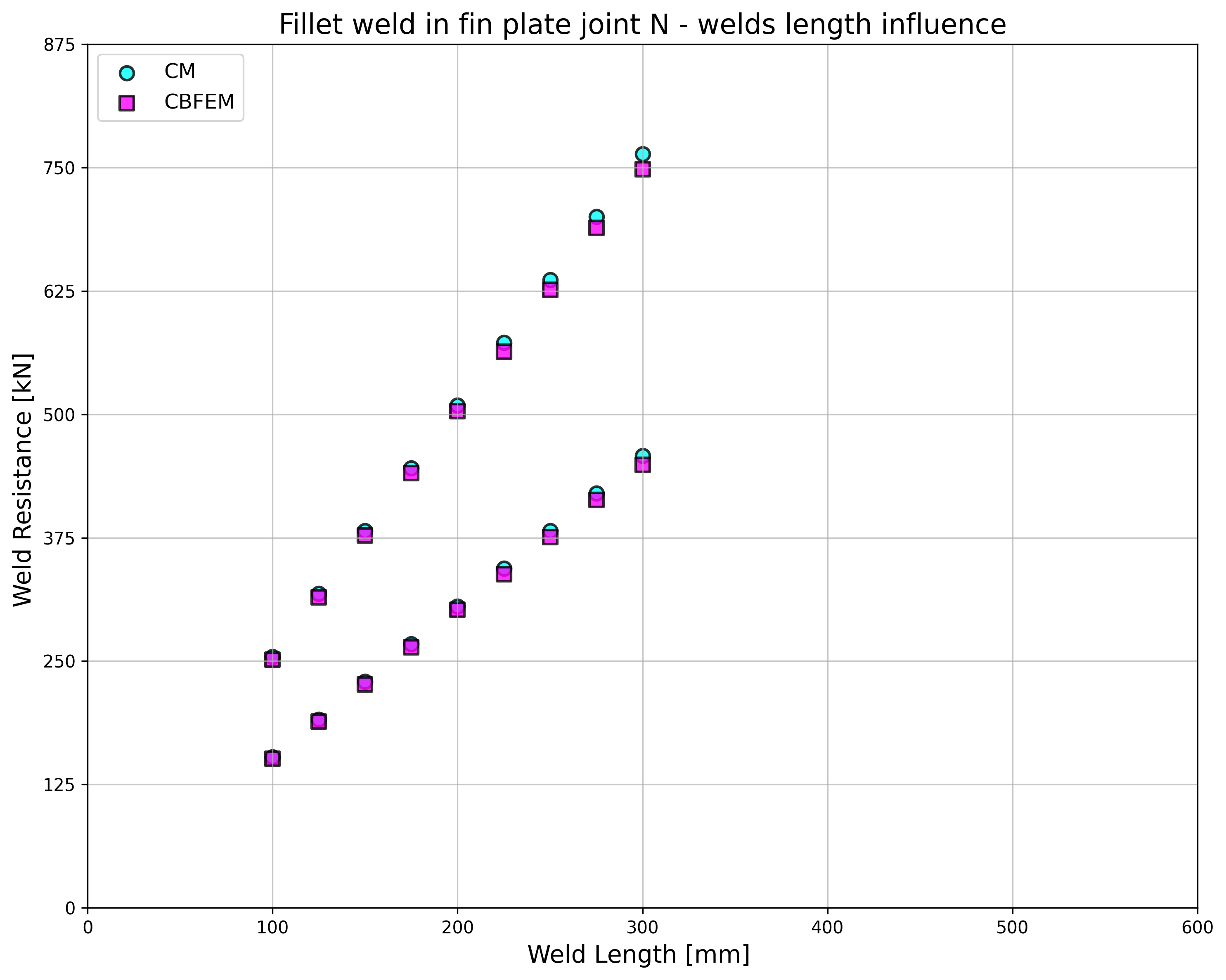
\[ \textsf{\textit{\footnotesize{Fig. 4.3.2 Parametric study of fin plate joint loaded by normal force}}}\]

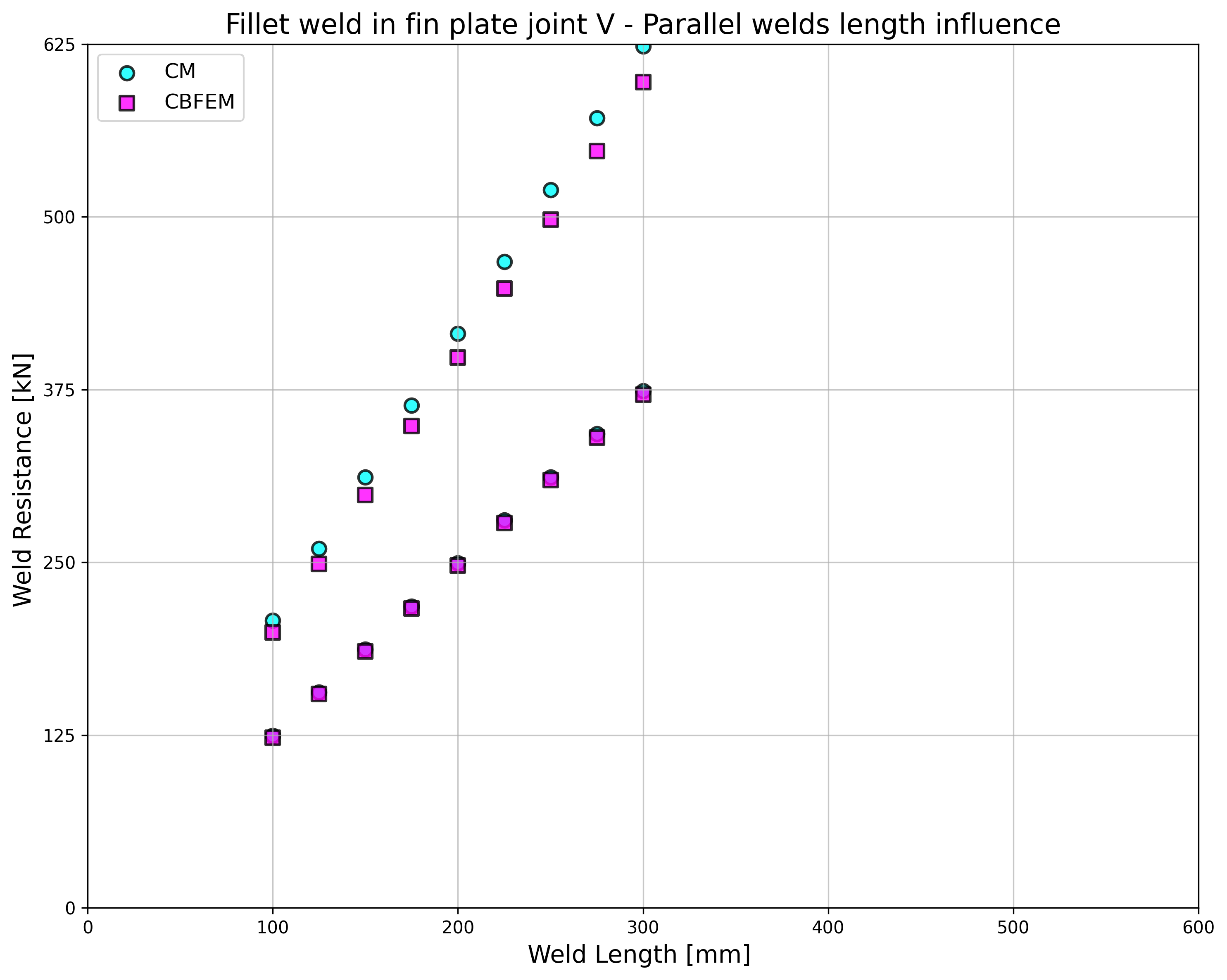
\[ \textsf{\textit{\footnotesize{Fig. 4.3.3 Parametric study of fin plate joint loaded by shear force}}}\]

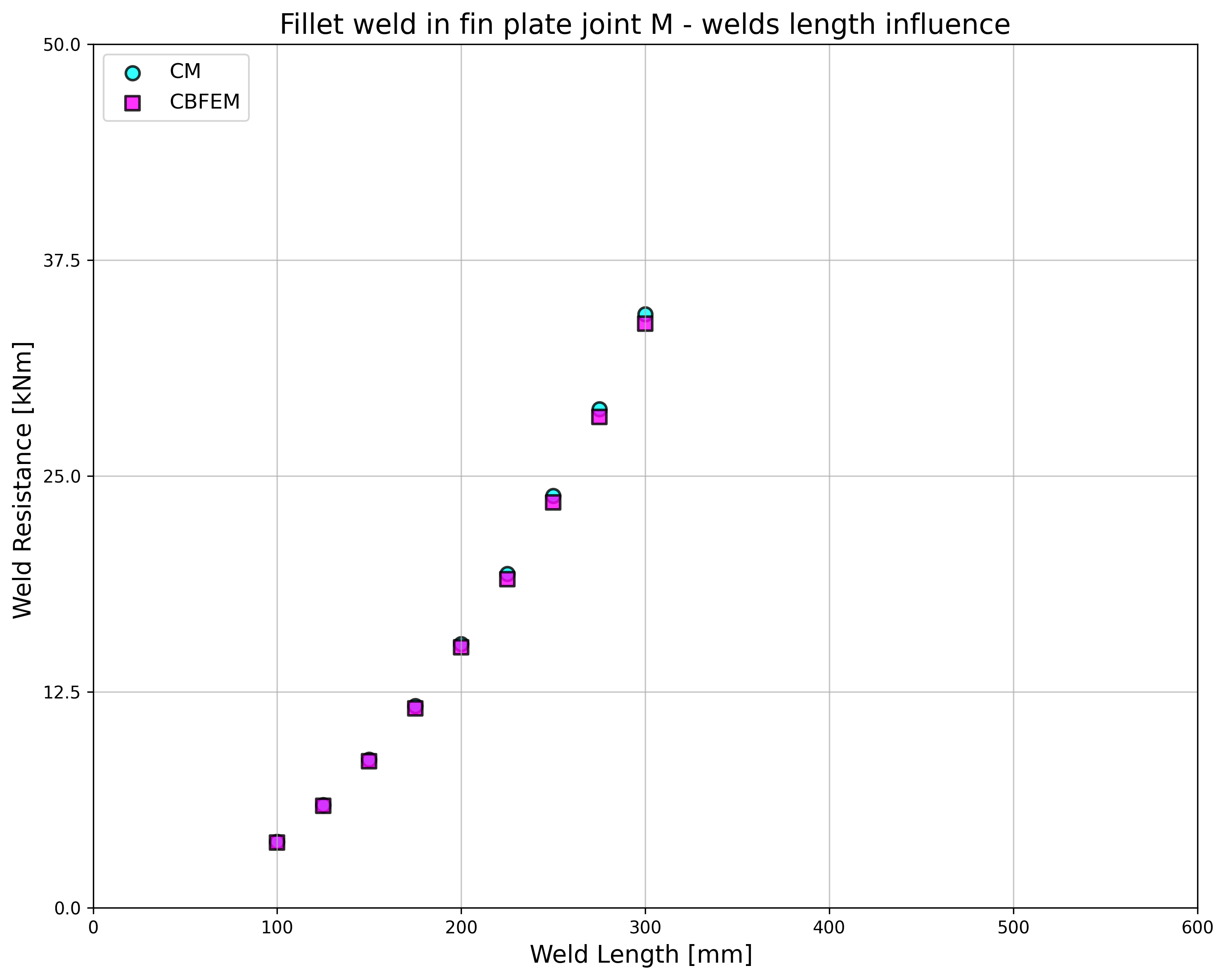
\[ \textsf{\textit{\footnotesize{Fig. 4.3.4 Parametric study of fin plate joint loaded by bending moment}}}\]

Pentru a ilustra acuratețea modelului CBFEM, rezultatele studiilor parametrice sunt rezumate într-un diagram care compară rezistențele de calcul ale CBFEM și CM; a se vedea Fig. 4.3.5. Rezultatele arată că diferența dintre cele două metode de calcul este în toate cazurile mai mică de 10 %.

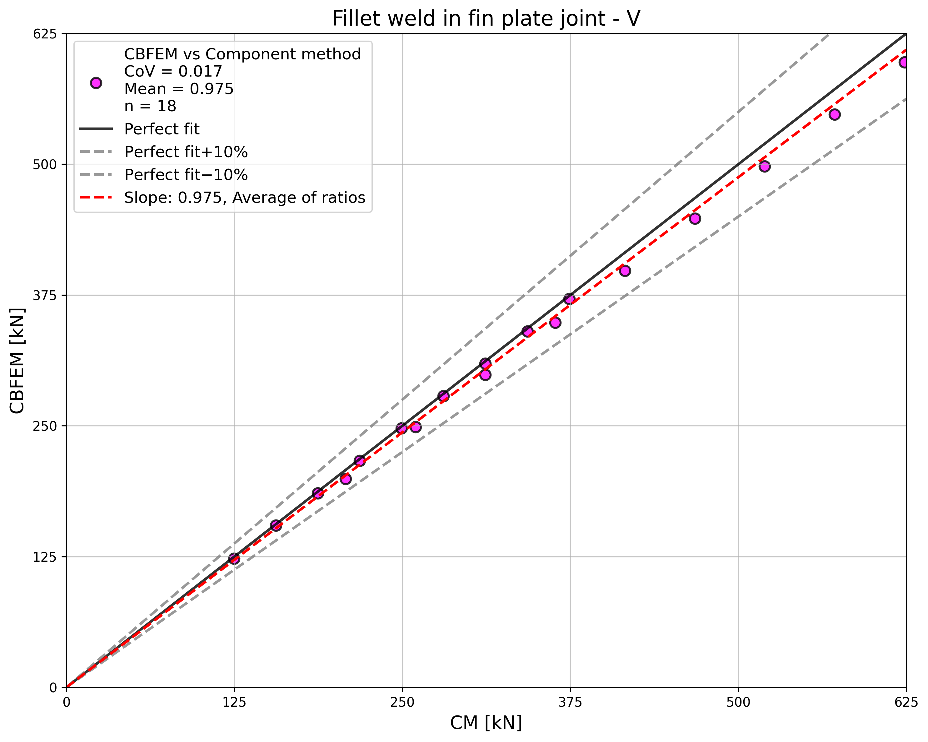
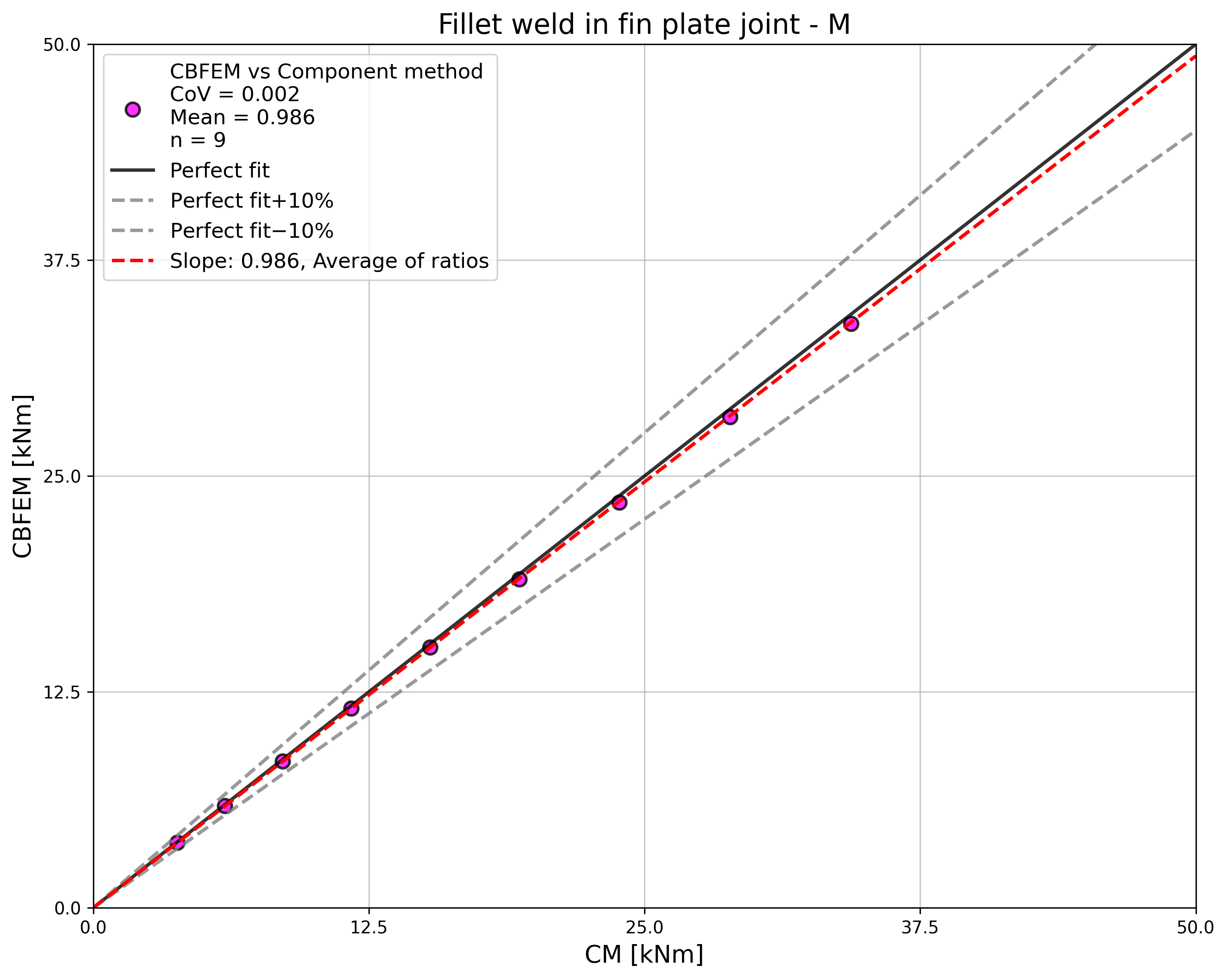
\[ \textsf{\textit{\footnotesize{Fig. 4.3.5 Verification of CBFEM to CM}}}\]

Exemplu de referință

Date de intrare

Stâlp

• Oțel S235
• HEB 400

Placă de inimă

• Grosime t_p = 15 mm
• Înălțime h_p = 175 mm

Sudură, sudură dublă de colț, a se vedea Fig. 4.3.6

• Grosimea gâtului a_w = 3 mm

Rezultate

• Rezistența de calcul la încovoiere pură M_Rd = 11,4 kNm

\[ \textsf{\textit{\footnotesize{Fig. 4.3.6 Benchmark example for the welded fin plate joint}}}\]

Sudură de colț în îmbinarea grindă-stâlp

 Descriere

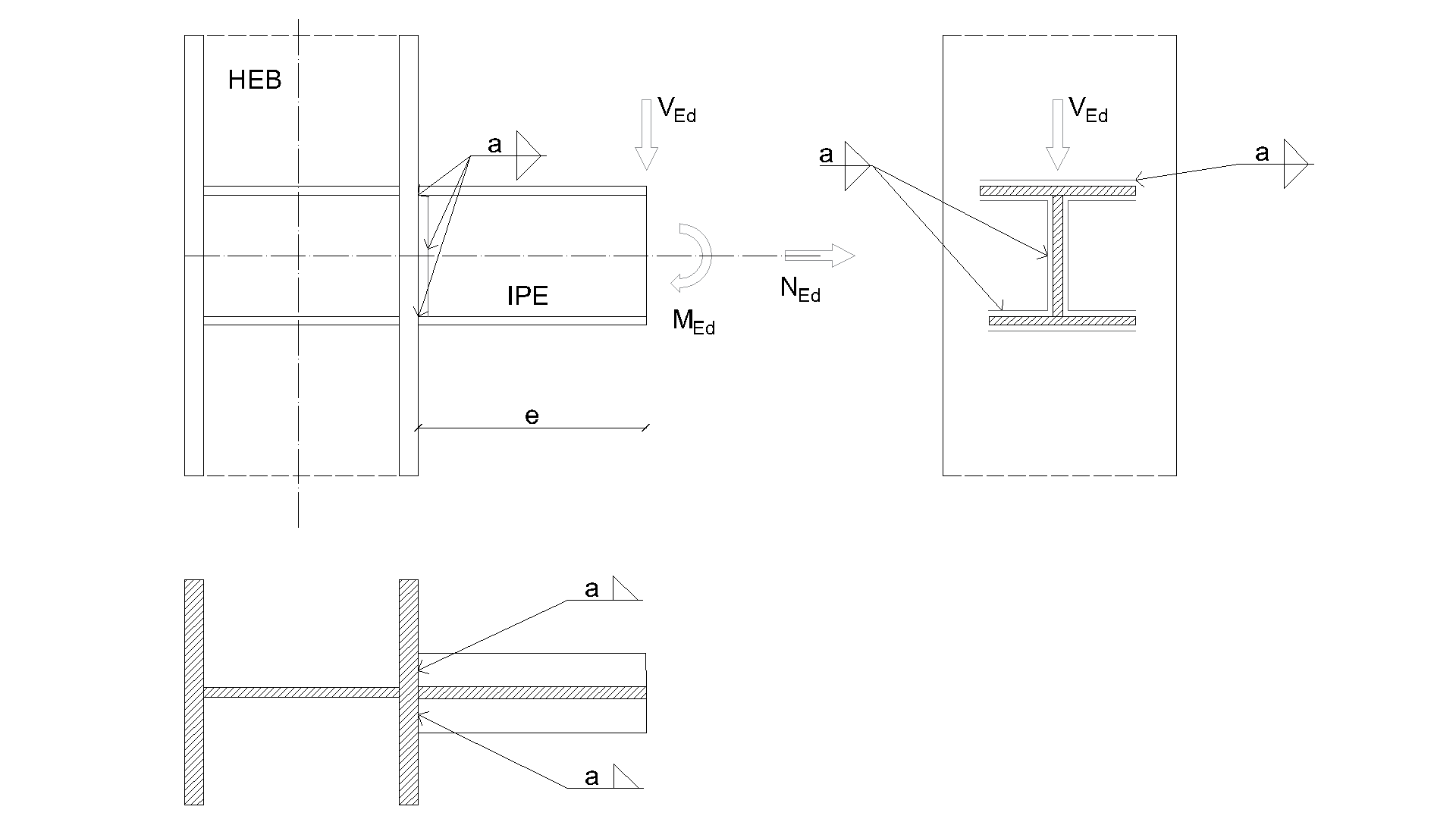
Obiectul acestui capitol este verificarea metodei elementelor finite bazate pe componente (CBFEM) pentru o sudură de colț într-o îmbinare grindă-stâlp cu rigidizări, prin metoda componentelor (CM). O grindă cu secțiune deschisă IPE este conectată la un stâlp cu secțiune deschisă HEB400. Rigidizările sunt amplasate în interiorul stâlpului, în dreptul tălpilor grinzii. Secțiunea grinzii este parametrul variabil. Sunt considerate trei cazuri de încărcare, respectiv grinda este încărcată la întindere, forfecare și încovoiere.

 Model analitic

Sudura de colț este singura componentă examinată în studiu. Sudurile sunt proiectate conform Capitolului 4 din EN 1993-1-8:2005 pentru a fi cea mai slabă componentă a îmbinării. Rezistența de calcul a sudurii de colț este descrisă în Secțiunea 4.1. Prezentarea generală a exemplelor considerate și a materialelor este dată în Tab. 4.4.1. Geometria îmbinării cu dimensiuni este prezentată în Fig. 4.4.1.

Tab. 4.4.1 Prezentarea generală a exemplelor

Calcul manual pentru forța normală N 

\[\sqrt{  \sigma_{\perp}^2  + 3 \cdot \left( \tau_{\perp}^2  + \tau_{\parallel}^2\right)} \leq \frac{f_u}{\beta_{\mathrm{w}} \cdot \gamma_{\mathrm{M2}}}\]

\[\sigma_{\perp} = \tau_{\perp} = \frac{\sigma_{N}}{\sqrt{2}} = \frac{N}{l \cdot a}\cdot \frac{1}{\sqrt{2}} \]

\[    \tau_{\parallel} = 0\]

\[    \sqrt{ \left( \frac{\sigma_{N}}{\sqrt{2}} \right)^2 + 3 \cdot \left( \frac{\sigma_{N}}{\sqrt{2}} \right)^2} \leq \frac{f_u}{\beta_{\mathrm{w}} \cdot \gamma_{\mathrm{M2}}}\]

\[    \sqrt{ \left( \frac{N}{l \cdot a}\cdot \frac{1}{\sqrt{2}} \right)^2 + 3 \cdot \left( \frac{N}{l \cdot a}\cdot \frac{1}{\sqrt{2}} \right)^2} \leq \frac{f_u}{\beta_{\mathrm{w}} \cdot \gamma_{\mathrm{M2}}}\]

\[ N \leq \frac{f_{u}  \cdot  l  \cdot  a }{\beta_{\mathrm{w}}  \cdot  \gamma_{\mathrm{M2}}  \cdot  \sqrt{2}} \]

Unde:

\(a\) - grosimea gâtului sudurii

\(N\) - forța normală care acționează pe grindă

\(l\) - lungimea totală a sudurilor 

\(\beta_{\mathrm{w}}\) - factor de corelație preluat din EN 1993-1-8 Tabelul 4.1

\(f_u\) - rezistența nominală la rupere prin întindere a elementului mai slab îmbinat

\(\gamma_{\mathrm{M2}}\) - factor parțial de siguranță pentru suduri

Calcul manual pentru forța tăietoare V 

Calculul manual prezentat în acest capitol se bazează pe anumite ipoteze. Forța tăietoare \(V\) este transmisă exclusiv prin sudura de pe inimă. Momentul încovoietor rezultat din excentricitatea forței care acționează pe suduri poate fi atribuit sudurilor de pe tălpi. Modulul de rezistență al secțiunii sudurii tălpilor \(W\) este determinat nu prin distanța măsurată față de centrul de greutate al sudurilor, ci față de marginile tălpii până la centrul de greutate al grinzii, conform practicii de calcul.

Ecuațiile următoare demonstrează derivarea capacității portante a sudurii pentru forța tăietoare și momentul încovoietor conform CM. Tensiunea echivalentă este specificată în EN 1993-1-8, Ecuația (4.1). Pentru calculul rezistenței la moment încovoietor, s-a adoptat modulul de rezistență plastic al secțiunii. 

\[\sqrt{  \sigma_{\perp}  + 3 \cdot \left( \tau_{\perp}^2  + \tau_{\parallel}^2\right)} \leq \frac{f_u}{\beta_{\mathrm{w}} \cdot \gamma_{\mathrm{M2}}}\]

\[V \le \min \left \{ \frac{f_\mathrm{u} \cdot l_V \cdot a}{\sqrt{3} \cdot \beta_{\mathrm{w}} \cdot \gamma_{M2}} , \,  \frac{f_\mathrm{u} \cdot W}{\sqrt{2} \cdot \beta_{\mathrm{w}} \cdot \gamma_{\mathrm{M2}} \cdot e}   \right \} \]

Unde:

\(e\) - excentricitatea forței față de sudurile grinzii 

\(a\) - grosimea gâtului sudurii

\(V\) - forța tăietoare care acționează pe grindă

\(W= W_\mathrm{pl,flange}\) - modulul de rezistență al secțiunii sudurilor

\(A_\mathrm{w,top,f} = B \cdot a\) - aria sudurii de margine a tălpii superioare 

\(A_\mathrm{w,bottom,f} = (B-t_\mathrm{w}) \cdot a\) - aria sudurii de margine a tălpii inferioare 

\(z_\mathrm{w,top,f} = H / 2 \) - brațul de pârghie al sudurii de margine a tălpii superioare

\(z_\mathrm{w,bottom,f} = (H - t_\mathrm{f}) / 2 \) - brațul de pârghie al sudurii de margine a tălpii inferioare

\(W_\mathrm{pl,flange} = 2 \cdot \left(A_\mathrm{w,top,f} \cdot  z_\mathrm{w,top,f} + A_\mathrm{w,bottom,f} \cdot z_\mathrm{w,bottom,f}\right)\) - modulul de rezistență plastic al secțiunii tălpilor

\(l_{\mathrm{V}}\) - lungimea totală a sudurilor de pe inimă 

\(\beta_{\mathrm{w}}\) - factor de corelație preluat din EN 1993-1-8 Tabelul 4.1

\(f_\mathrm{u}\) - rezistența nominală la rupere prin întindere a elementului mai slab îmbinat

\(\gamma_{\mathrm{M2}}\) - factor parțial de siguranță pentru suduri

\(H\) - înălțimea grinzii IPE

\(B\) - lățimea grinzii IPE

\(t_\mathrm{w}\) - grosimea inimii grinzii IPE 

\(t_\mathrm{f}\) - grosimea tălpii grinzii IPE

Calcul manual pentru momentul încovoietor M

La calculul momentului încovoietor fără interacțiune cu forța tăietoare, s-a adoptat modulul de rezistență plastic al întregii secțiuni a sudurii (atât în jurul tălpilor, cât și în jurul inimii).

\[\sqrt{ \sigma_{\perp}^2 + 3 \cdot \left( \tau_{\perp}^2 + \tau_{\parallel}^2\right)} \leq \frac{f_u}{\beta_{\mathrm{w}} \cdot \gamma_{\mathrm{M2}}}\]

\[\sigma_{\perp} = \tau_{\perp} = \frac{\sigma_{N}}{\sqrt{2}} = \frac{M}{W}\cdot \frac{1}{\sqrt{2}} \]

\[ \tau_{\parallel} = 0\]

\[ \sqrt{ \left( \frac{\sigma_{N}}{\sqrt{2}} \right)^2 + 3 \cdot \left( \frac{\sigma_{N}}{\sqrt{2}} \right)^2} \leq \frac{f_u}{\beta_{\mathrm{w}} \cdot \gamma_{\mathrm{M2}}}\]

\[ \sqrt{ \left( \frac{M}{W}\cdot \frac{1}{\sqrt{2}} \right)^2 + 3 \cdot \left( \frac{M}{W}\cdot \frac{1}{\sqrt{2}} \right)^2} \leq \frac{f_u}{\beta_{\mathrm{w}} \cdot \gamma_{\mathrm{M2}}}\]

\[ M \leq \frac{f_{u} \cdot W }{\beta_{\mathrm{w}}  \cdot  \gamma_{\mathrm{M2}}  \cdot  \sqrt{2}} \]

\[ \sigma_{\perp} \leq \frac{f_{u}  \cdot  0.9}{ \gamma_{\mathrm{M2}}} \]

\[ M \leq \frac{f_{u}  \cdot  W  \cdot  0.9  \cdot  \sqrt{2}}{ \gamma_{\mathrm{M2}} }   \]

Unde:

\(a\) - grosimea gâtului sudurii

\(W \) - modulul de rezistență plastic al secțiunii sudurii

\(M\) - momentul încovoietor care acționează pe grindă

\(\beta_{\mathrm{w}}\) - factor de corelație preluat din EN 1993-1-8 Tabelul 4.1

\(f_u\) - rezistența nominală la rupere prin întindere a elementului mai slab îmbinat

\(\gamma_{\mathrm{M2}}\) - factor parțial de siguranță pentru suduri

 Model numeric

Componenta de sudură în CBFEM este descrisă în Fundamente teoretice generale și Fundamente teoretice EN. 

În acest studiu se utilizează un material elastic-plastic neliniar pentru suduri. Deformația plastică limită este atinsă pe o porțiune mai lungă a sudurii, iar concentrările de tensiuni sunt redistribuite.

\[ \textsf{\textit{\footnotesize{Fig. 4.4.1 Geometria îmbinării cu dimensiuni}}}\]

 Verificarea rezistenței

Rezistența de calcul calculată cu software-ul CBFEM Idea RS este comparată cu rezultatele CM. Rezistențele de calcul ale sudurilor sunt comparate, a se vedea Tab. 4.4.2. Studiul este realizat pentru un parametru de secțiune a grinzii și trei cazuri de încărcare: forță normală N_Ed, forță tăietoare V_Ed și moment încovoietor M_Ed.

Tab. 4.4.2 Comparație între CBFEM și CM

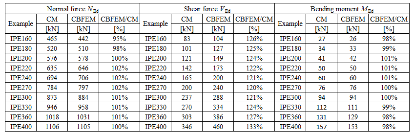
Rezultatele CBFEM și CM sunt comparate și este prezentată un studiu de sensibilitate. Influența secțiunii transversale a grinzii asupra rezistenței de calcul a unei îmbinări grindă-stâlp sudate, încărcată la întindere, este prezentată în Fig. 4.4.2, la forfecare în Fig. 4.4.3 și la încovoiere în Fig. 4.4.4. Studiul arată o concordanță bună pentru toate cazurile de încărcare aplicate.

\[ \textsf{\textit{\footnotesize{Fig. 4.4.2}}}\]

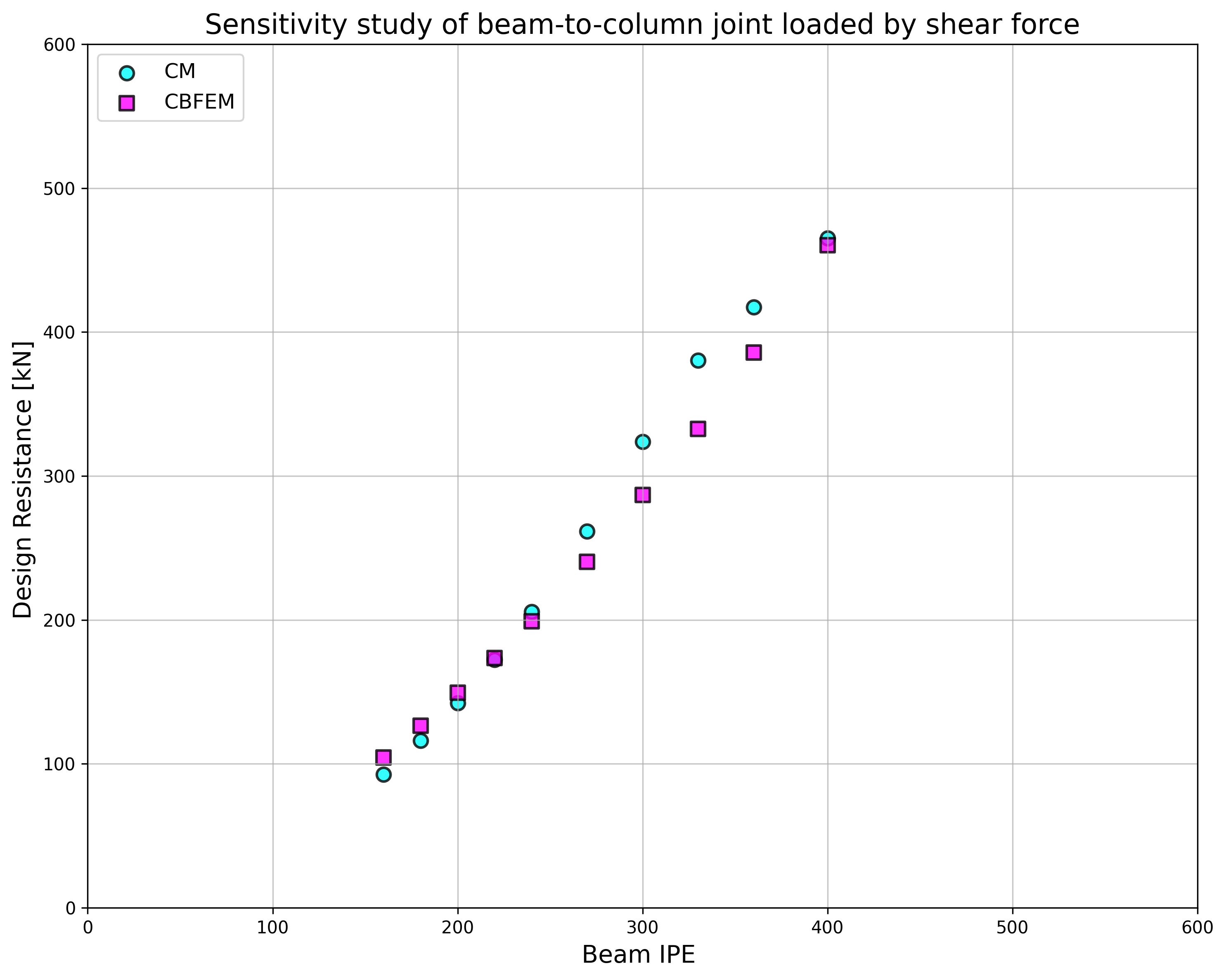
\[ \textsf{\textit{\footnotesize{Fig. 4.4.3}}}\]

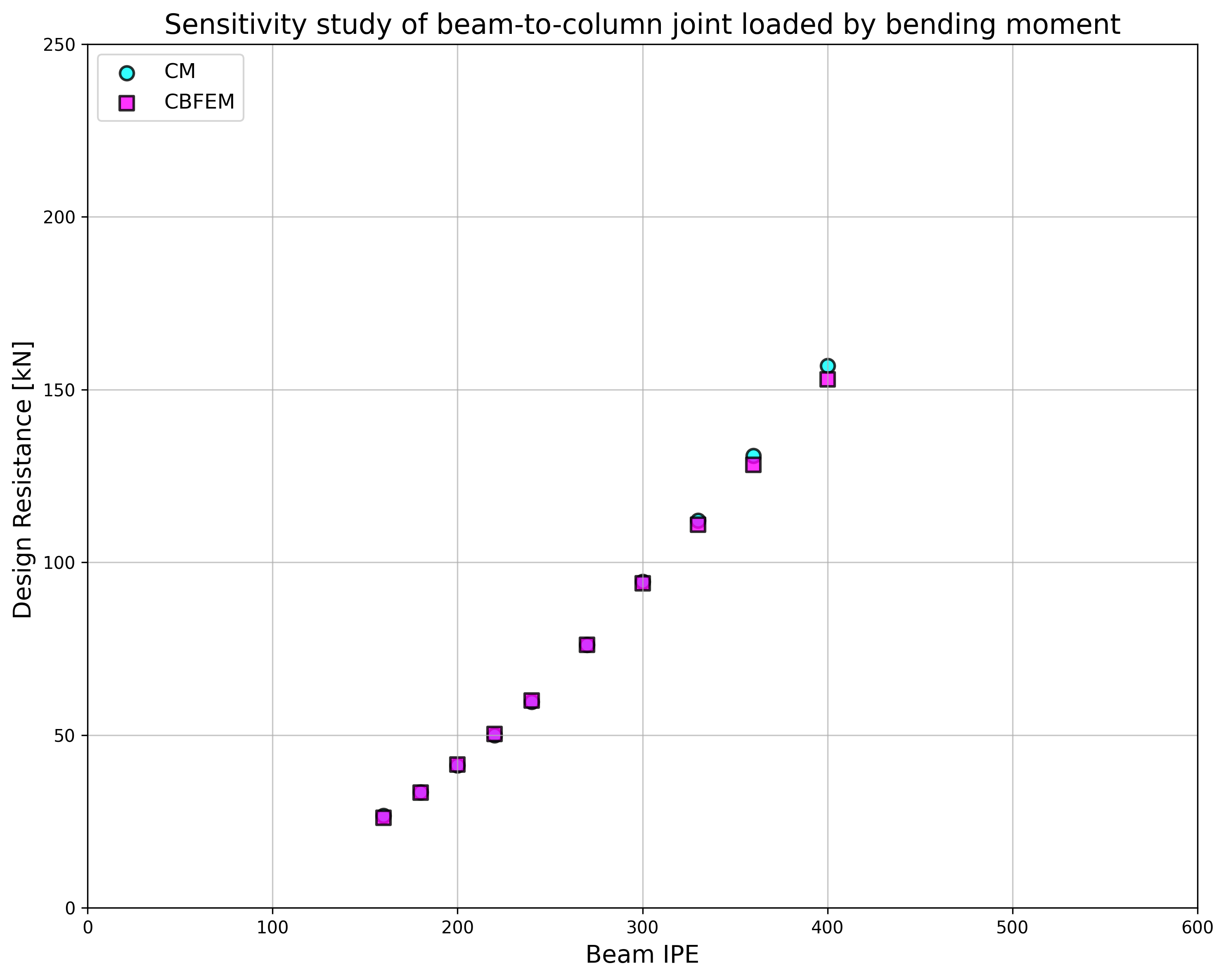
\[ \textsf{\textit{\footnotesize{Fig. 4.4.4}}}\]

Pentru a ilustra acuratețea modelului CBFEM, rezultatele studiului de sensibilitate sunt rezumate într-un diagram care compară rezistențele de calcul ale CBFEM și CM, a se vedea Fig. 4.4.5. Rezultatele arată că diferența dintre cele două metode de calcul este în toate cazurile mai mică de 10%.

\[ \textsf{\textit{\footnotesize{Fig. 4.4.5 Verificarea CBFEM față de CM}}}\]

 Exemplu de referință

Date de intrare

Stâlp

• Oțel S235
• HEB 400

Grindă

•  Oțel S235
•  IPE 160
•  Excentricitatea forței față de sudură x = 400 mm, a se vedea Fig. 4.4.6

Sudură

•   Grosimea gâtului a_w = 3 mm

Date de ieșire:

• Rezistența de calcul la forfecare V_Rd = 105 kN

\[ \textsf{\textit{\footnotesize{Fig. 4.4.6 Exemplu de referință al îmbinării grindă-stâlp sudate cu excentricitatea forței}}}\]

Îmbinare la tălpi nerigidizate

Descriere

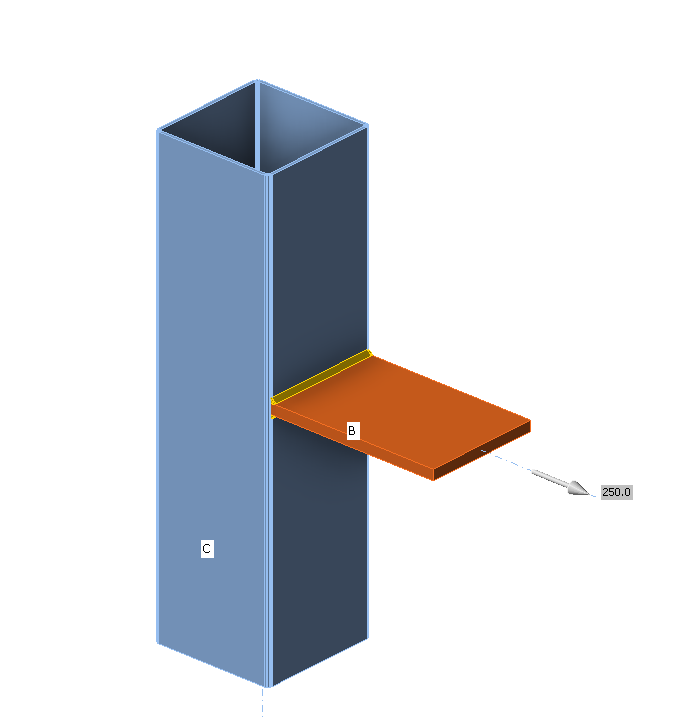
În acest capitol, metoda elementelor finite bazată pe componente (CBFEM) pentru o sudură de colț care conectează o placă la o talpă nerigidizată de stâlp este verificată prin metoda componentelor (CM). Placa metalică este conectată la stâlpi cu secțiune deschisă și secțiune casetată și este încărcată la întindere.

Model analitic

Sudura de colț este singura componentă examinată în studiu. Sudurile sunt proiectate conform Capitolului 4 din EN 1993-1-8:2005 pentru a fi componenta cea mai slabă din îmbinare. Rezistența de calcul a sudurii de colț este descrisă în Secțiunea 4.1. Forța aplicată perpendicular pe o placă flexibilă, sudată la o secțiune nerigidizată, este limitată. Tensiunile sunt concentrate într-o lățime efectivă, în timp ce rezistența sudurii în dreptul părților nerigidizate este neglijată, conform Fig. 4.5.1. Pentru o secțiune I sau H nerigidizată, lățimea efectivă se obține conform:

\[ b_\mathrm{eff} = t_\mathrm{w} + 2s + 7kt_\mathrm{f} \qquad (4.5.1)\]                                                                    

\[ k = \frac{t_\mathrm{f} \cdot f_\mathrm{y,f} }{ t_\mathrm{p} \cdot f_\mathrm{y,p}} \qquad (4.5.2)\]                                                         

Dimensiunea s este pentru o secțiune laminată \(s =r\) și pentru o secțiune sudată \(s = \sqrt{2} \cdot a \) . Pentru o secțiune casetată sau U, lățimea efectivă se obține din:

\[ b_\mathrm{eff} = 2t_\mathrm{w} + 5 t_\mathrm{f} \quad \textrm{but}\quad b_\mathrm{eff} \leq 2t_\mathrm{w} + 5 kt_\mathrm{f}\qquad (4.5.1)\] 

\[\sqrt{  \sigma_{\perp}^2  + 3 \cdot \left( \tau_{\perp}^2  + \tau_{\parallel}^2\right)} \leq \frac{f_u}{\beta_{\mathrm{w}} \cdot \gamma_{\mathrm{M2}}}\]

\[\sigma_{\perp} = \tau_{\perp} = \frac{\sigma_{N}}{\sqrt{2}} = \frac{N}{b_\mathrm{eff} \cdot a}\cdot \frac{1}{\sqrt{2}} \]

\[    \tau_{\parallel} = 0\]

\[    \sqrt{ \left( \frac{\sigma_{N}}{\sqrt{2}} \right)^2 + 3 \cdot \left( \frac{\sigma_{N}}{\sqrt{2}} \right)^2} \leq \frac{f_u}{\beta_{\mathrm{w}} \cdot \gamma_{\mathrm{M2}}}\]

\[    \sqrt{ \left( \frac{N}{b_\mathrm{eff} \cdot a}\cdot \frac{1}{\sqrt{2}} \right)^2 + 3 \cdot \left( \frac{N}{b_\mathrm{eff}\cdot a}\cdot \frac{1}{\sqrt{2}} \right)^2} \leq \frac{f_u}{\beta_{\mathrm{w}} \cdot \gamma_{\mathrm{M2}}}\]

\[ N \leq \frac{f_{u}  \cdot  b_\mathrm{eff}  \cdot  a }{\beta_{\mathrm{w}}  \cdot  \gamma_{\mathrm{M2}}  \cdot  \sqrt{2}} \]

Unde:

\(a\) - grosimea gâtului sudurii

\(N\) - forța normală care acționează pe grindă

\(b_\mathrm{eff}\) - lungimea totală efectivă a sudurilor 

\(\beta_{\mathrm{w}}\) - factor de corelație preluat din Tabelul 4.1 al EN 1993-1-8

\(f_u\) - rezistența nominală la rupere prin întindere a elementului mai slab îmbinat

\(\gamma_{\mathrm{M2}}\) - factor parțial de siguranță pentru suduri

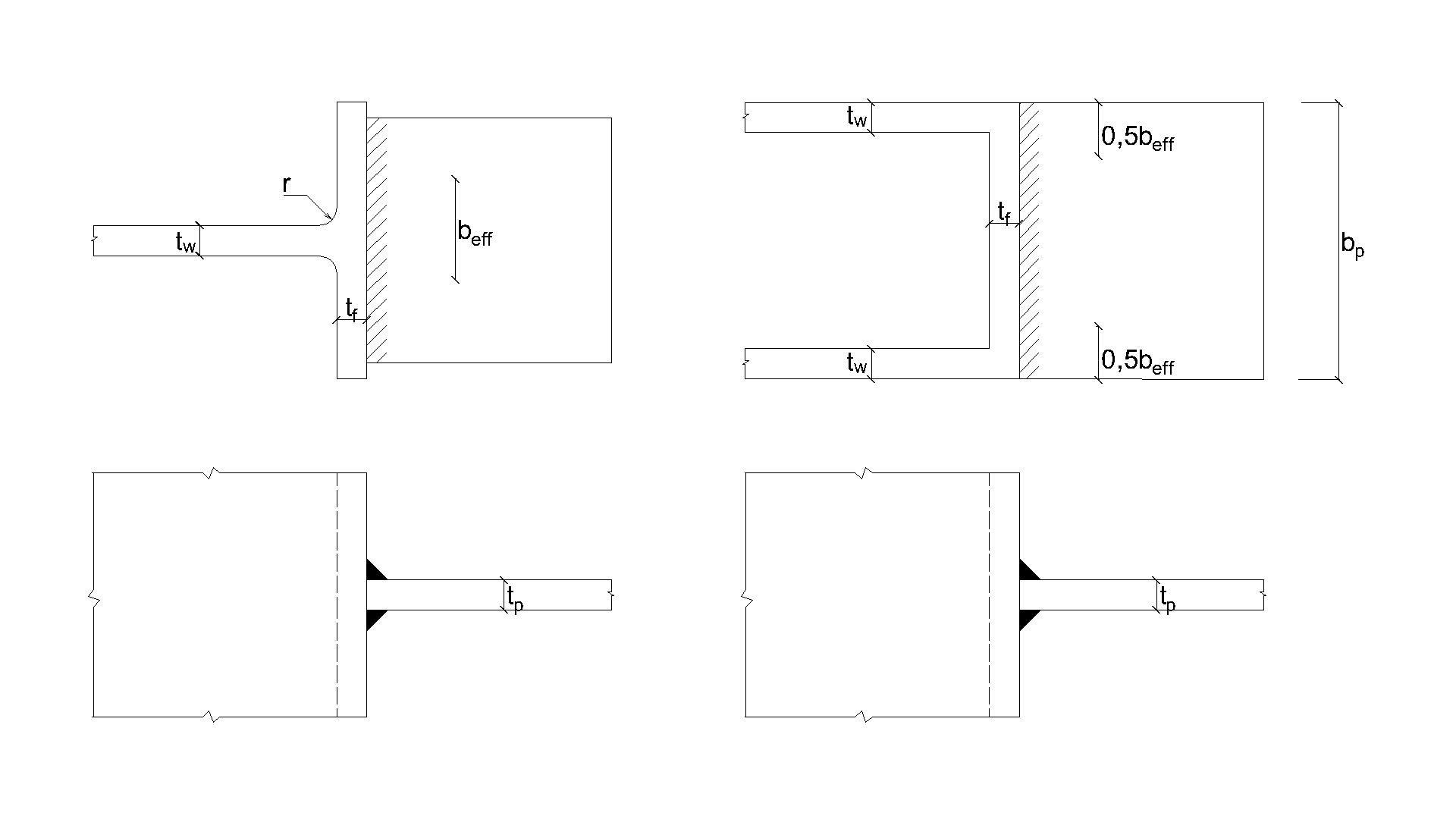
       \[ \textsf{\textit{\footnotesize{Fig. 4.5.1 Lățimea efectivă a unei îmbinări nerigidizate (Fig. 4.8 din EN 1993-1-8:2005)}}}\]

Model numeric

Componenta de sudură în CBFEM este descrisă în Fundamente teoretice generale și Fundamente teoretice EN. Ramura plastică este atinsă într-o parte a sudurii, iar vârfurile de tensiune sunt redistribuite de-a lungul lungimii sudurii.

Verificarea rezistenței

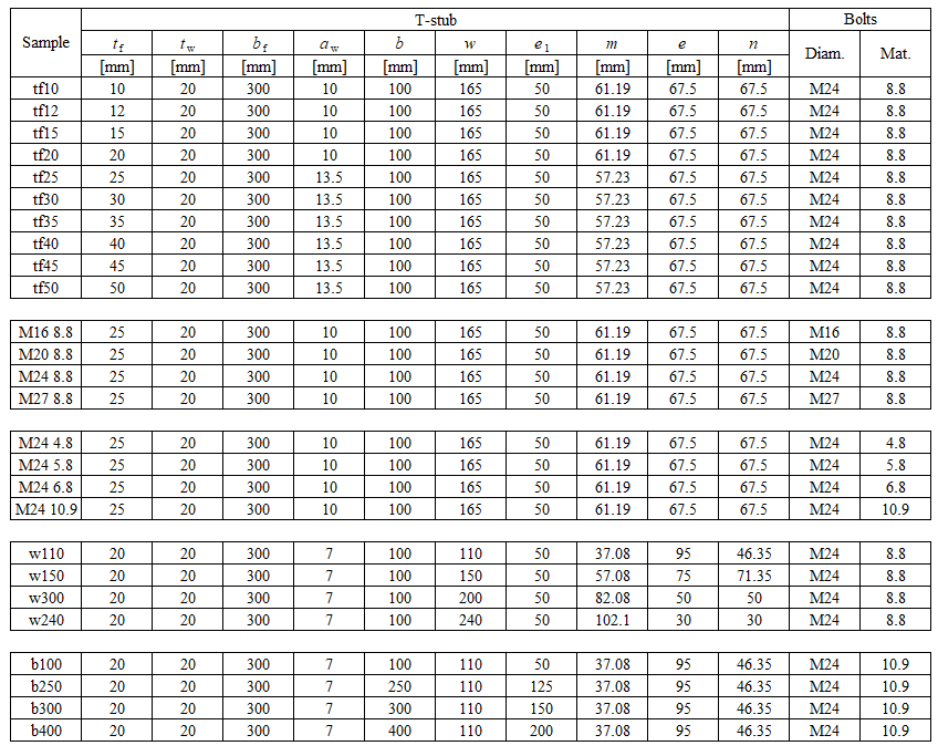
Rezistența de calcul calculată prin CBFEM este comparată cu rezultatele CM. Se compară doar rezistența de calcul a sudurii. Prezentarea generală a exemplelor considerate și a materialelor este dată în Tab. 4.5.1. Geometria îmbinărilor cu dimensiuni este prezentată în Fig. 4.5.2.

\[ \textsf{\textit{\footnotesize{Tab. 4.5.1 Prezentarea generală a exemplelor}}}\]

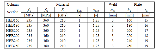
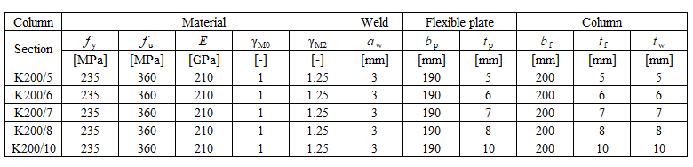
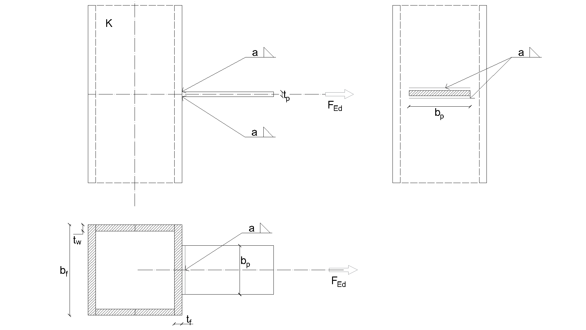
\[ \textsf{\textit{\footnotesize{a) Placă flexibilă la secțiune deschisă             b) Placă flexibilă la secțiune casetată}}}\]

\[ \textsf{\textit{\footnotesize{Fig. 4.5.2 Geometria și dimensiunile îmbinării}}}\]

Rezultatele sunt prezentate în Tab. 4.5.2. Studiul este realizat pentru doi parametri: lățimea tălpii secțiunii HEB și grosimea inimii secțiunii caseta. Placa flexibilă este încărcată la întindere. Influența lățimii tălpii secțiunii HEB asupra rezistenței de calcul a îmbinării este prezentată în Fig. 4.5.3. Relația dintre grosimea inimii secțiunii caseta și rezistența de calcul a îmbinării este prezentată în Fig. 4.5.4.

\[ \textsf{\textit{\footnotesize{Tab. 4.5.2 Comparație între CBFEM și CM}}}\]

Rezultatele CBFEM și CM sunt comparate într-un studiu de sensibilitate. Influența lățimii tălpii secțiunii HEB asupra rezistenței de calcul a îmbinării este studiată în Fig. 4.5.3. Influența grosimii inimii secțiunii caseta asupra rezistenței de calcul a îmbinării este prezentată în Fig. 4.5.4. Studiile parametrice arată o concordanță foarte bună a rezultatelor pentru toate configurațiile de suduri.

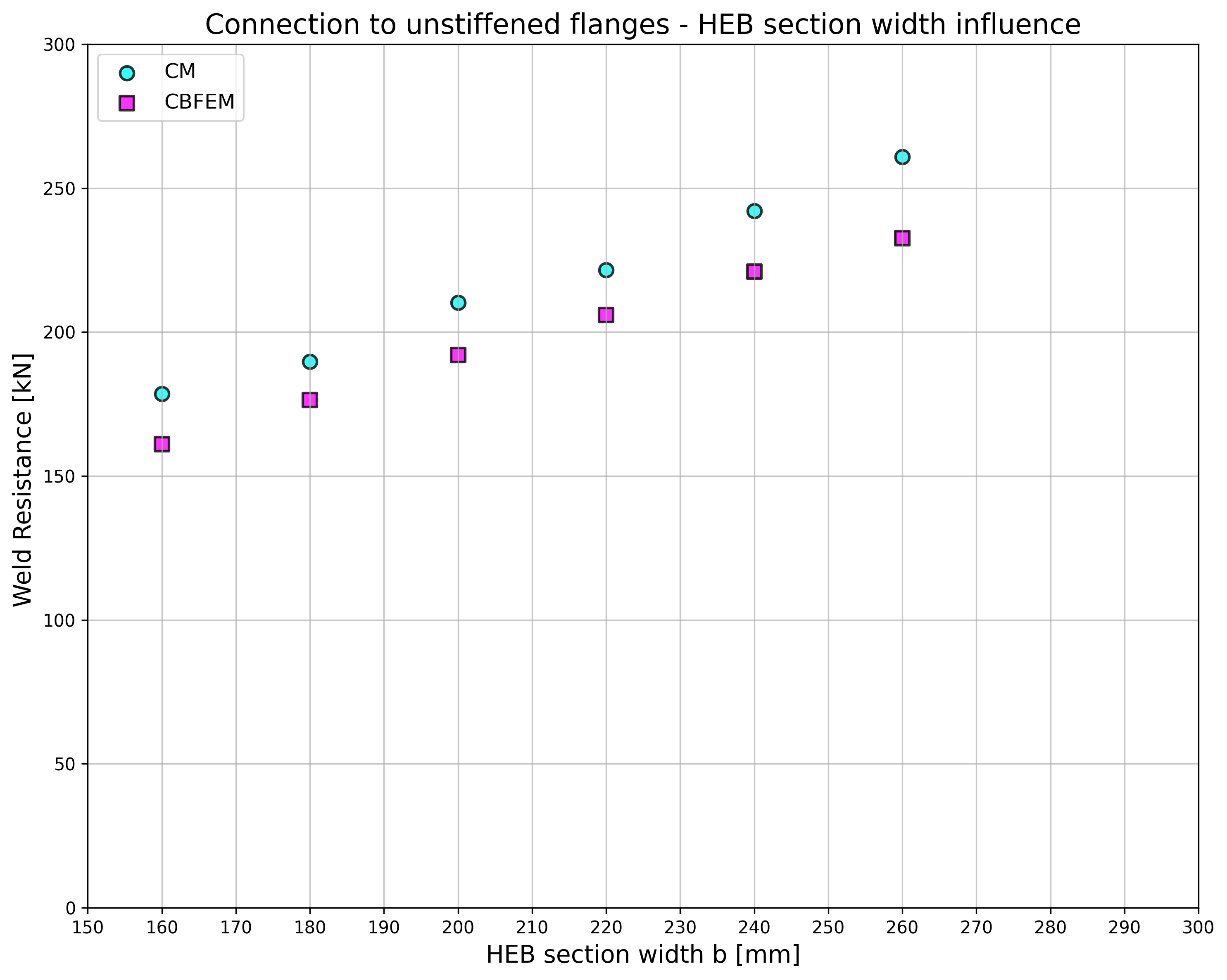
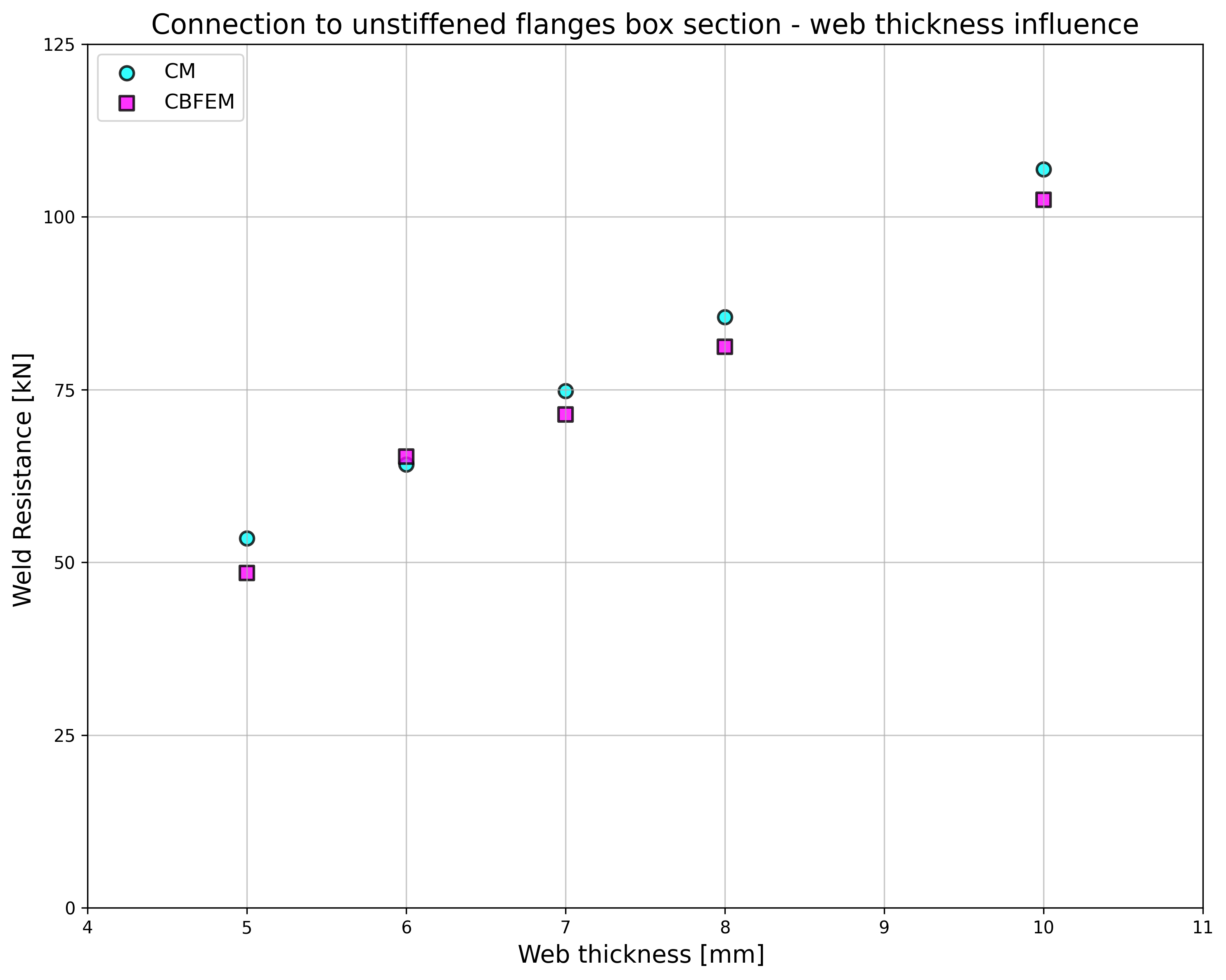
\[ \textsf{\textit{\footnotesize{Fig. 4.5.3 Lățimea tălpii secțiunii HEB      Fig. 4.5.4 Grosimea inimii secțiunii caseta}}}\]

Rezultatele studiului de sensibilitate sunt rezumate într-un diagram care compară rezistențele de calcul ale CBFEM și CM; a se vedea Fig. 4.5.5 care ilustrează acuratețea modelului CBFEM.

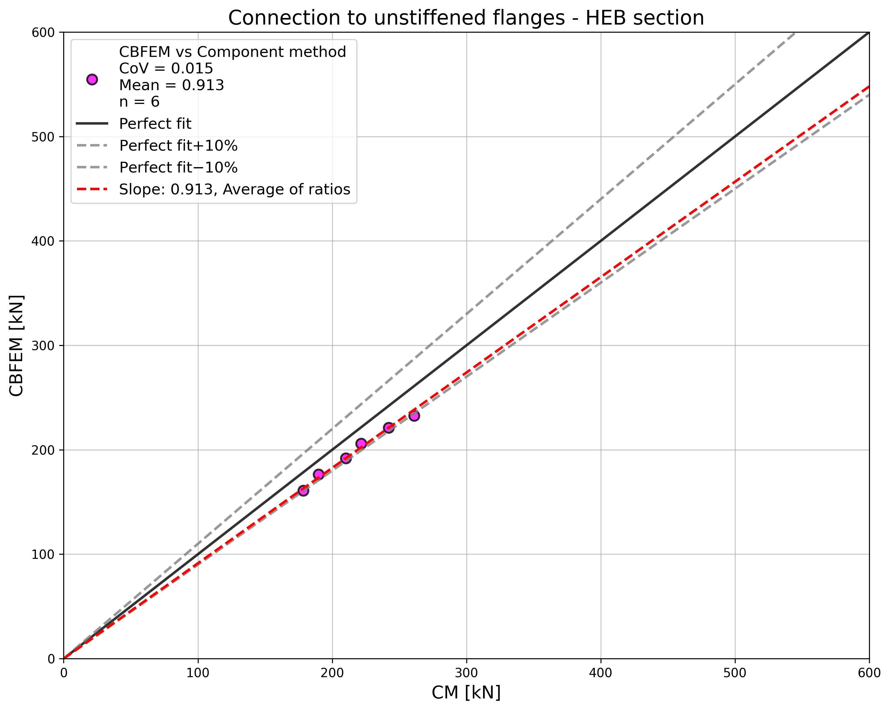
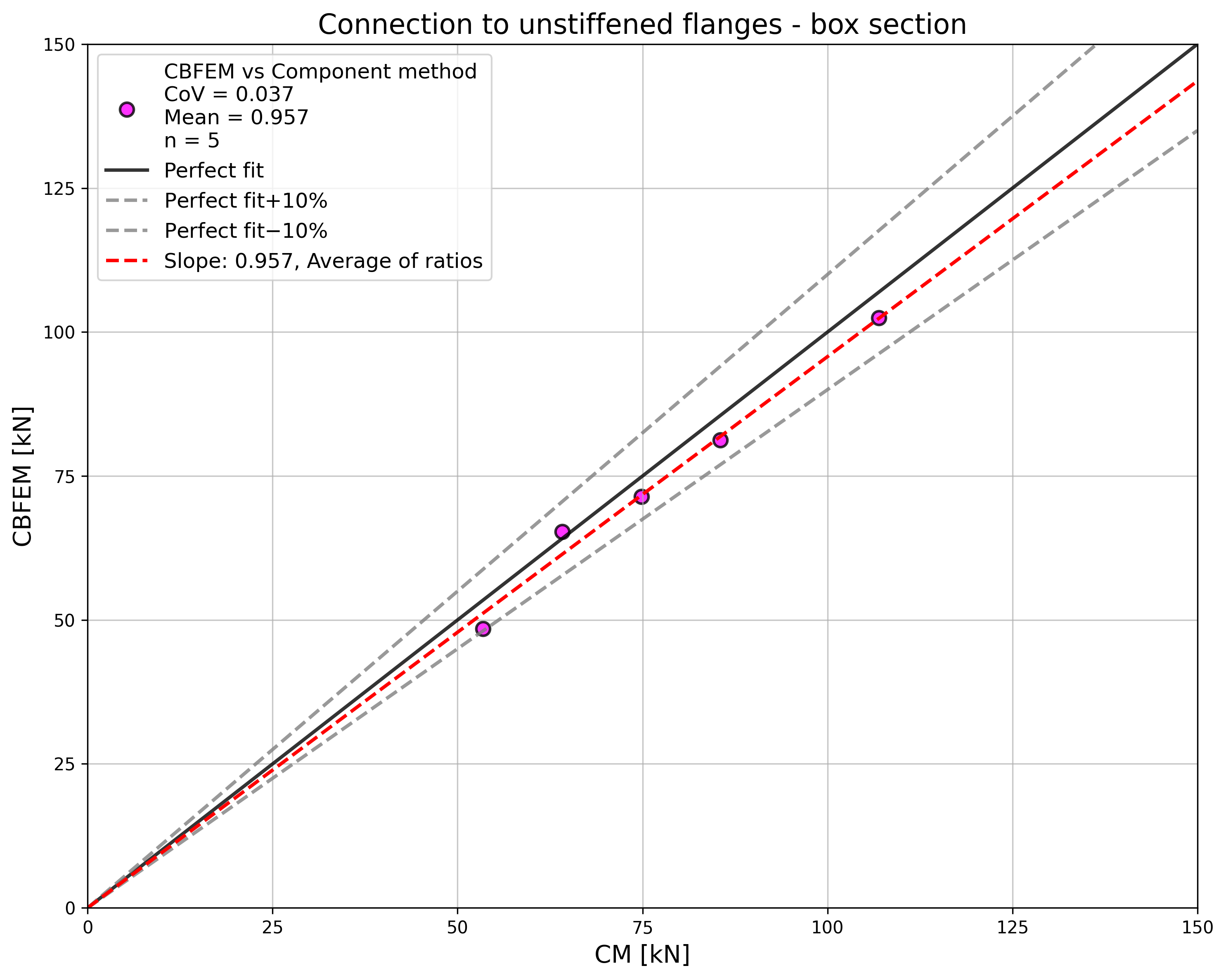
\[ \textsf{\textit{\footnotesize{Fig. 4.5.5 Verificarea CBFEM față de CM}}}\]

Influența grosimii plăcii asupra rezistenței de calcul a sudurii este prezentată în Fig. 4.5.6. Secțiunea transversală a stâlpului este HEB 180 cu o grosime a tălpii de 14 mm. O sudură care conectează o placă mai groasă decât talpa stâlpului are aceeași rezistență pentru CM și CBFEM. Pe de altă parte, sudura care conectează placa la talpa stâlpului de aceeași grosime sau mai mică are în modelele numerice o rezistență de calcul mai mică cu 20%. Grosimea plăcii nu este luată în considerare în modelele numerice cu elemente de tip placă, ceea ce cauzează diferența.

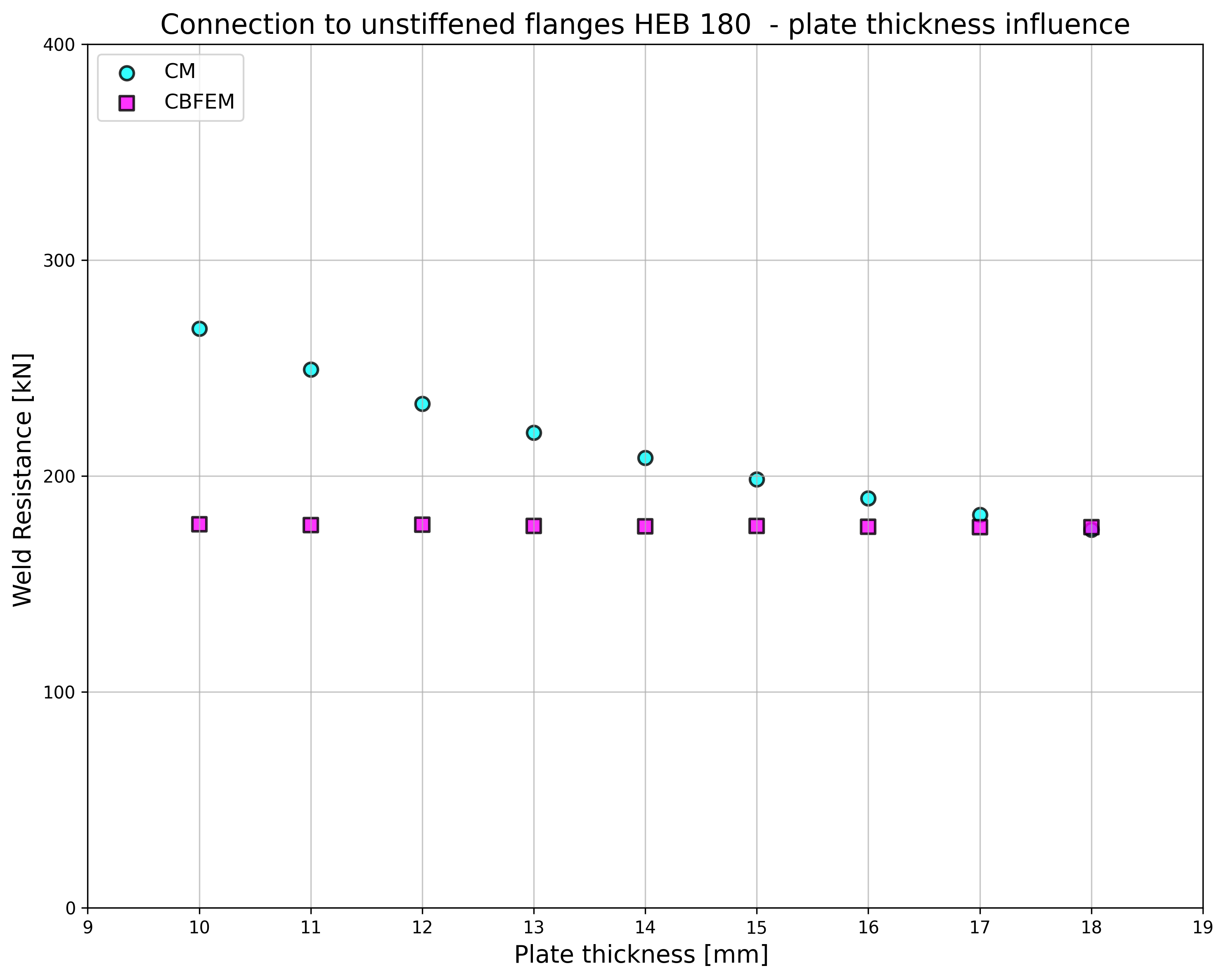
\[ \textsf{\textit{\footnotesize{Fig. 4.5.6 Influența grosimii plăcii asupra rezistenței îmbinării cu stâlp nerigidizat HEB180}}}\]

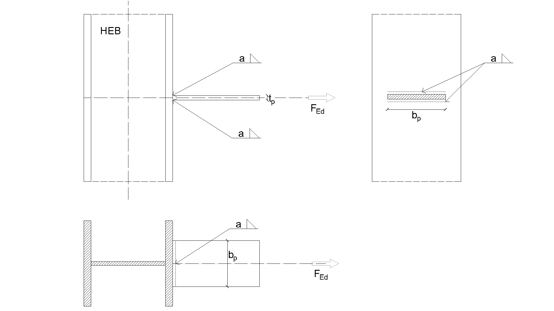
Exemplu de referință

Date de intrare

Stâlp

• Oțel S235

• RHS 200/200/5

Placă flexibilă

• Oțel S235

• Grosime t_p = 17 mm

• Lățime b_p = 190 mm

Sudură, suduri duble de colț, a se vedea Fig. 4.5.7

• Grosimea gâtului a_w = 5 mm

Rezultate

• Rezistența de calcul la întindere N_Rd = 68 kN

\[ \textsf{\textit{\footnotesize{Fig. 4.5.7 Exemplu de referință pentru îmbinarea sudată a plăcii la stâlpul nerigidizat}}}\]

Îmbinări cu șuruburi 

Îmbinare cu șuruburi - T-stub în întindere

Descriere

Obiectivul acestui capitol este verificarea metodei cu elemente finite bazate pe componente (CBFEM) pentru T-stub-uri conectate cu două șuruburi încărcate în întindere, prin comparație cu metoda componentelor (CM) și modelul FEM de cercetare (RM) creat în software-ul Midas FEA; a se vedea (Gödrich et al. 2019).

Model analitic

T-stub-ul sudat și șurubul în întindere sunt componentele examinate în studiu. Ambele componente sunt proiectate conform EN 1993-1-8:2005. Sudurile sunt proiectate astfel încât să nu fie componenta cea mai slabă. Lungimile efective pentru cedările circulare și necirculare sunt considerate conform EN 1993-1-8:2005 cl. 6.2.6. Se iau în considerare doar încărcări de întindere. Trei moduri de cedare conform EN 1993-1-8:2005 cl. 6.2.4.1 sunt considerate: 1. modul cu plastifierea completă a tălpii, 2. modul cu două linii de plastifiere la inimă și ruperea șuruburilor, și 3. modul pentru ruperea șuruburilor; a se vedea Fig. 5.1.1. Șuruburile sunt proiectate conform cl. 3.6.1 din EN 1993-1-8:2005. Rezistența de calcul ia în considerare rezistența la forfecare prin poansonare și ruperea șurubului.

\[ \textsf{\textit{\footnotesize{Fig. 5.1.1 Collapse modes of T-stub}}}\]

Model numeric de calcul

T-stub-ul este modelat cu elemente de tip placă cu 4 noduri, după cum este descris în Capitolul 3 și rezumat în continuare. Fiecare nod are 6 grade de libertate. Deformațiile elementului constau din contribuții membranare și de încovoiere. Starea elastoplastică neliniară a materialului este investigată în fiecare strat al punctului de integrare. Evaluarea se bazează pe deformația maximă dată conform EN 1993‑1‑5:2006 prin valoarea de 5 %. Șuruburile sunt împărțite în trei sub-componente. Prima este tija șurubului, care este modelată ca un arc neliniar și preia doar întindere. A doua sub-componentă transmite forța de întindere în tălpi. A treia sub-componentă rezolvă transmiterea forței de forfecare.

Model numeric de cercetare

În cazurile în care CBFEM oferă o rezistență mai mare, o rigiditate inițială mai mare sau o capacitate de deformație mai mare, modelul FEM de cercetare (RM) din elemente solide, validat pe experimente (Gödrich et al. 2013), este utilizat pentru verificarea modelului CBFEM. RM este creat în software-ul Midas FEA din elemente solide hexaedrice și octaedrice, a se vedea Fig. 5.1.2. Un studiu de sensibilitate a plasei a fost efectuat pentru a obține rezultate corecte într-un timp adecvat. Modelul numeric al șuruburilor se bazează pe modelul lui (Wu et al. 2012). Diametrul nominal este considerat în tijă, iar diametrul efectiv al miezului este considerat în partea filetată. Șaibele sunt cuplate cu capul și piulița. Deformația cauzată de dezfiletarea filetelor în zona de contact filet–piuliță este modelată folosind elemente de interfață. Elementele de interfață nu pot transfera tensiuni de întindere. Elementele de contact care permit transmiterea presiunii și frecării sunt utilizate între șaibe și tălpile T-stub-ului. Un sfert din eșantion a fost modelat folosind simetria.

\[ \textsf{\textit{\footnotesize{Fig. 5.1.2 Research FEM model}}}\]

\[ \textsf{\textit{\footnotesize{Fig. 5.1.3 Geometry of the T-stubs}}}\]

Domeniu de valabilitate

CBFEM a fost verificat pentru geometrii tipice selectate ale T-stub-ului. Grosimea minimă a tălpii este de 8 mm. Distanța maximă dintre șuruburi față de diametrul șurubului este limitată de p/d_b ≤ 20. Distanța liniei de șuruburi față de inimă este limitată la m/d_b ≤ 5. Prezentarea generală a eșantioanelor considerate cu plăci de oțel S235: f_y = 235 MPa, f_u = 360 MPa, E = E_bolt = 210 GPa este prezentată în Tab. 5.1.1 și în Fig. 5.1.3.

Tab. 5.1.1 Prezentare generală a eșantioanelor considerate de T-stub-uri

Comportament global

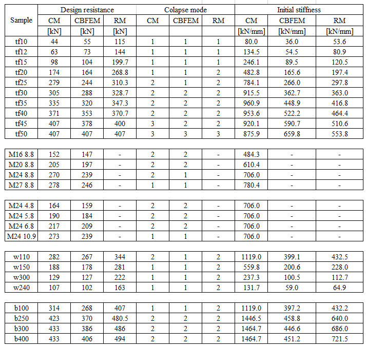
A fost pregătită o comparație a comportamentului global al T-stub-ului descris prin diagrame forță–deformație pentru toate procedurile de calcul. Atenția a fost concentrată pe caracteristicile principale: rigiditate inițială, rezistență de calcul și capacitate de deformație. Eșantionul tf20 a fost ales ca referință; a se vedea Fig. 5.1.4 și Tab. 5.1.2. CM oferă în general o rigiditate inițială mai mare comparativ cu CBFEM și RM. În toate cazurile, RM oferă cea mai mare rezistență de calcul, după cum se arată în capitolul 6. Capacitatea de deformație este de asemenea comparată. Capacitatea de deformație a T-stub-ului a fost calculată conform (Beg et al. 2004). RM nu ia în considerare fisurarea materialului, astfel că predicția capacității de deformație este limitată.

\[ \textsf{\textit{\footnotesize{Fig. 5.1.4 Force–deformation diagram}}}\]

Tab. 5.1.2 Prezentare generală a comportamentului global

Verificarea rezistenței

Rezistențele de calcul calculate prin CBFEM au fost comparate cu rezultatele CM și RM în etapa următoare. Comparația a fost axată și pe capacitatea de deformație și determinarea modului de cedare. Toate rezultatele sunt ordonate în Tab. 5.1.3. Studiul a fost efectuat pentru cinci parametri: grosimea tălpii, dimensiunea șurubului, materialul șurubului, distanța dintre șuruburi și lățimea T-stub-ului.

Tab. 5.1.3 Prezentare generală a comportamentului global

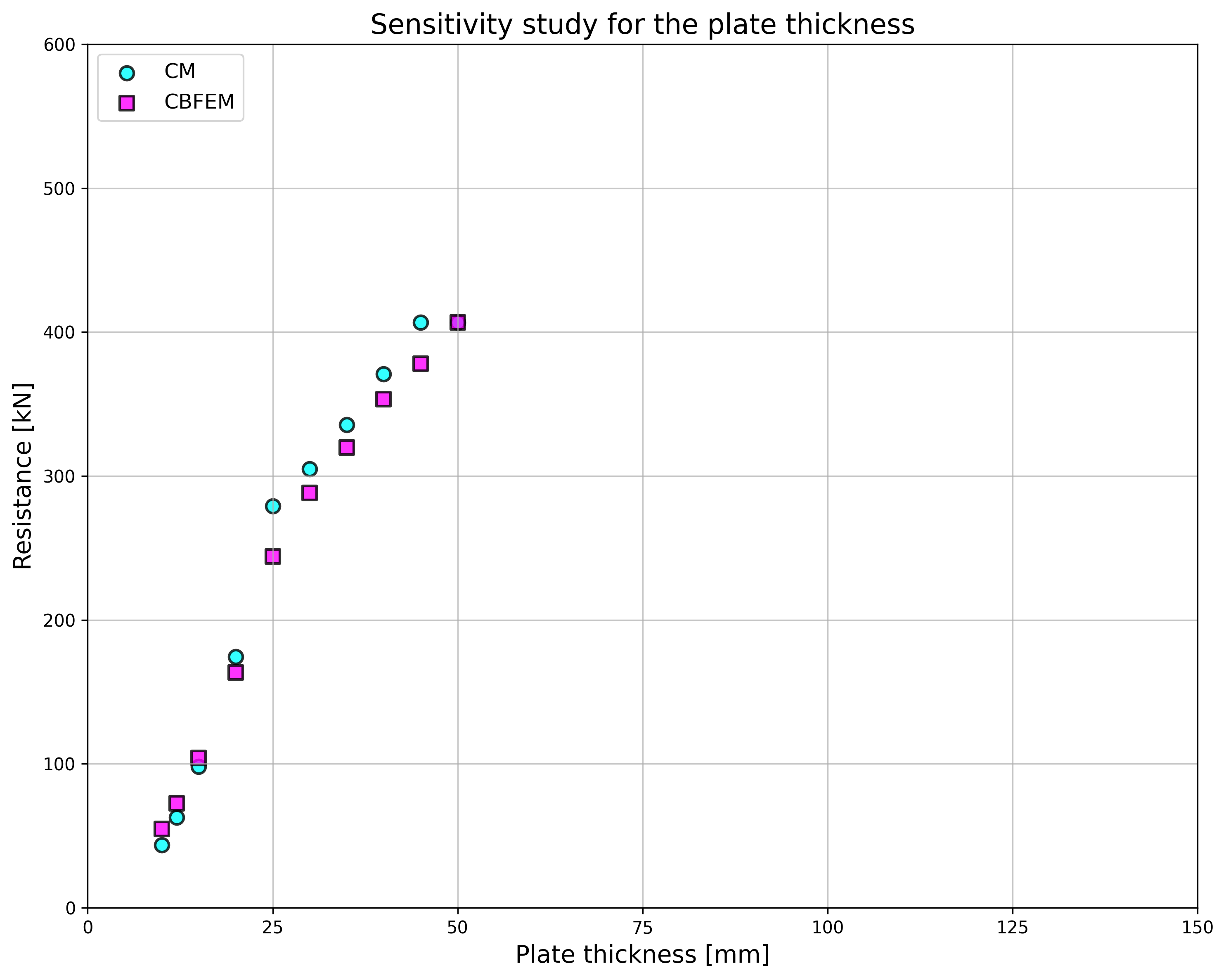
\[ \textsf{\textit{\footnotesize{Fig. 5.1.5 Sensitivity study of flange thickness}}}\]

Studiul de sensibilitate al grosimii tălpii arată o rezistență mai mare conform CBFEM comparativ cu CM pentru eșantioanele cu grosimi ale tălpii de până la 20 mm. RM oferă o rezistență și mai mare pentru aceste eșantioane; a se vedea Fig. 5.1.5. Rezistența mai mare a ambelor modele numerice este explicată prin neglijarea efectului membranar în CM. În cazul diametrului șurubului și al materialului șurubului (a se vedea Fig. 5.1.6 și respectiv Fig. 5.1.7), rezultatele CBFEM corespund celor din CM. Datorită bunei concordanțe dintre cele două metode, rezultatele RM nu sunt necesare.

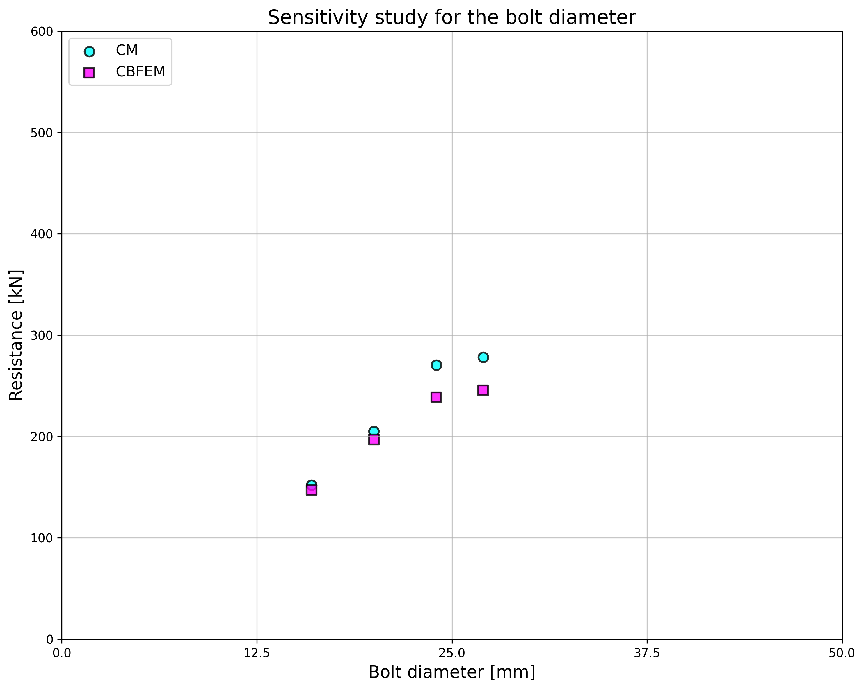
\[ \textsf{\textit{\footnotesize{Fig. 5.1.6 Sensitivity study of the bolt diameter}}}\]

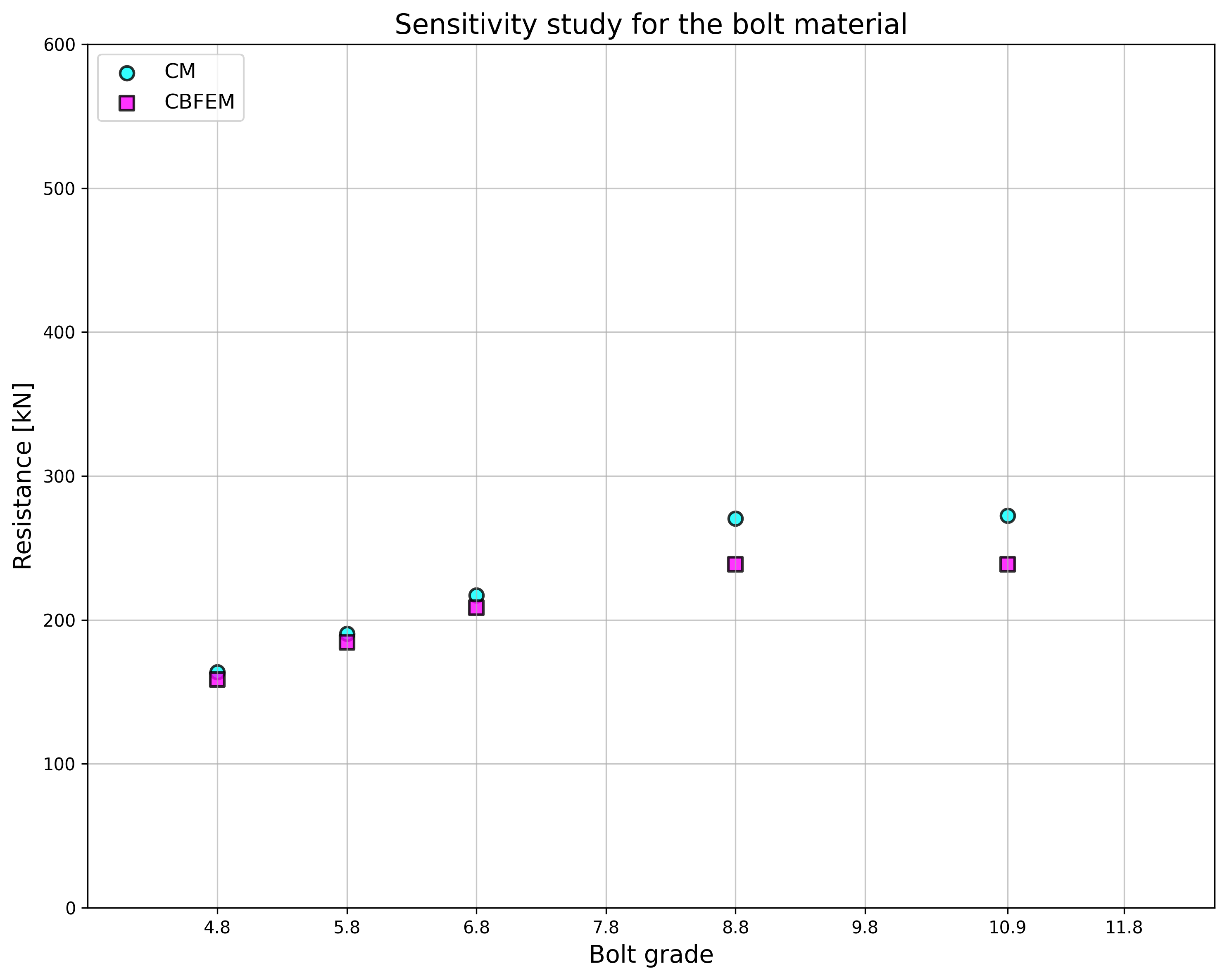
\[ \textsf{\textit{\footnotesize{Fig. 5.1.7 Sensitivity study of the bolt material}}}\]

În cazul distanțelor dintre șuruburi, rezultatele CBFEM și CM arată în general o bună concordanță; a se vedea Fig. 5.1.8. Odată cu creșterea distanței dintre șuruburi, CBFEM oferă o rezistență ușor mai mare comparativ cu CM. Din acest motiv, sunt prezentate și rezultatele RM. RM oferă cea mai mare rezistență în toate cazurile.

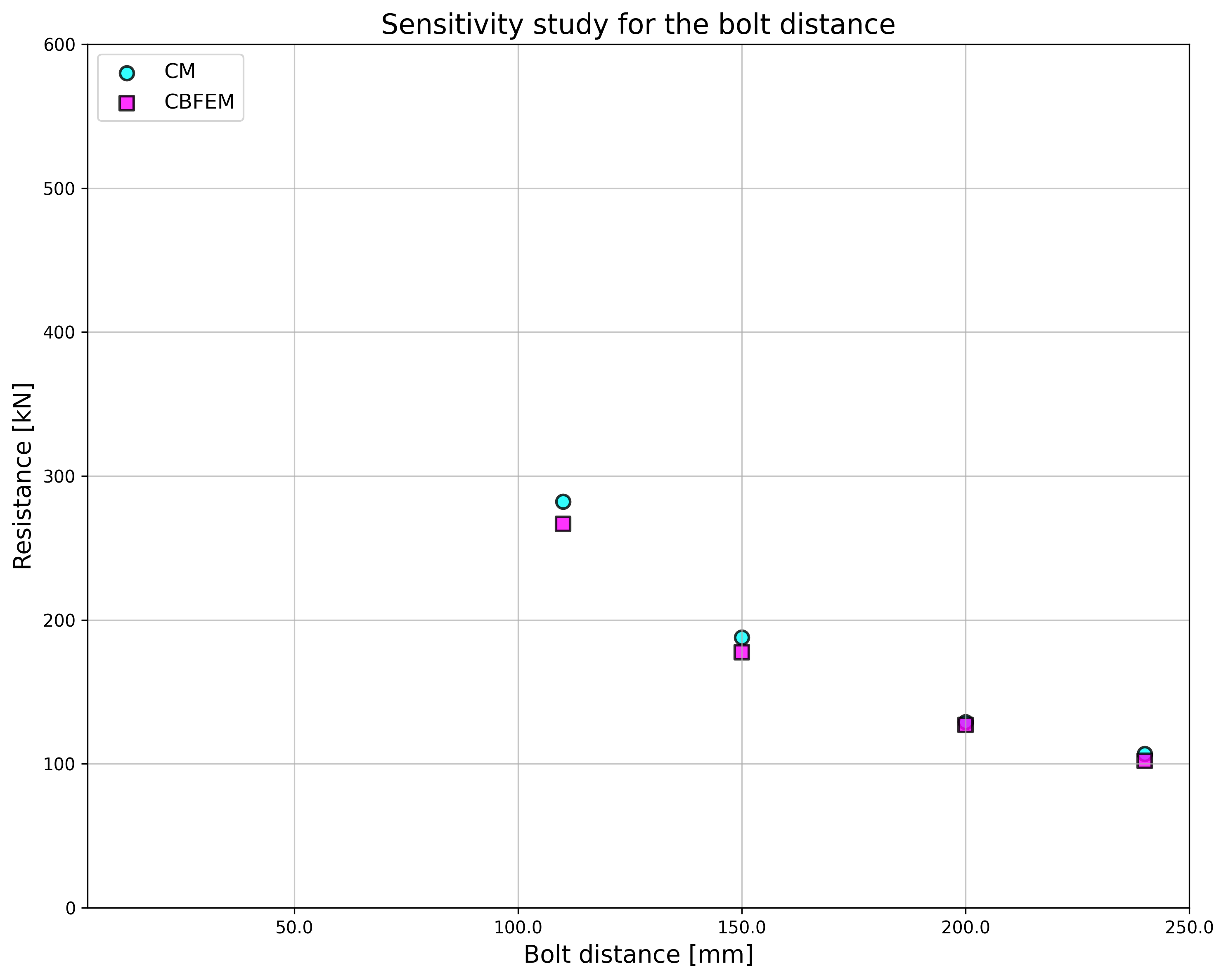
\[ \textsf{\textit{\footnotesize{Fig. 5.1.8 Sensitivity study of the bolt distance}}}\]

În studiul lățimii T-stub-ului, CBFEM arată o rezistență mai mare comparativ cu CM odată cu creșterea lățimii. Au fost pregătite rezultatele RM, care oferă din nou cea mai mare rezistență în toate cazurile; a se vedea Fig. 5.1.9.

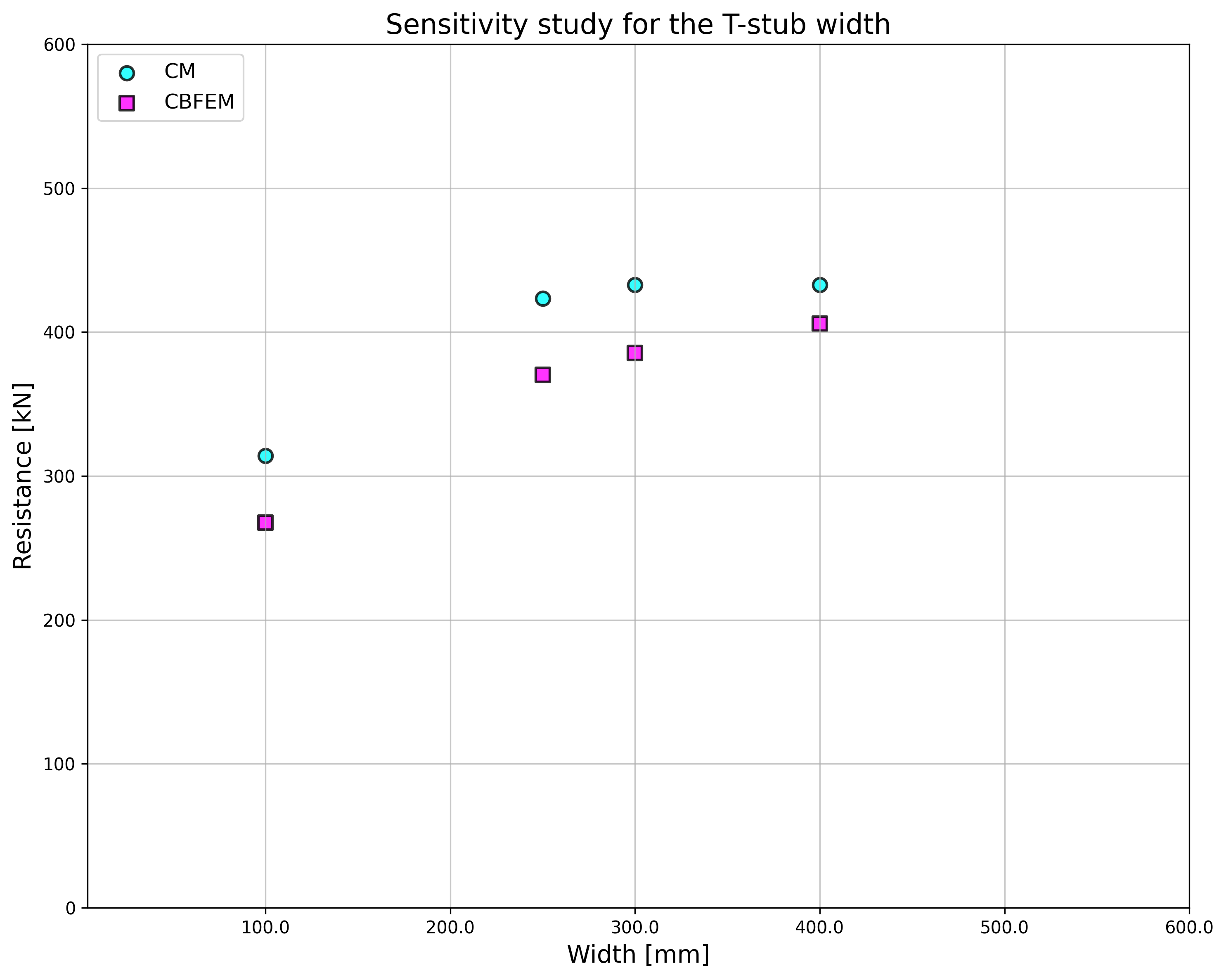
\[ \textsf{\textit{\footnotesize{Fig. 5.1.9 Sensitivity study of T-stub width}}}\]

Pentru a prezenta predicția modelului CBFEM, rezultatele studiilor au fost rezumate într-un grafic care compară rezistențele obținute prin CBFEM și CM; a se vedea Fig. 5.1.10. Rezultatele arată că diferența dintre cele două metode de calcul este în cea mai mare parte de până la 10 %. În cazurile cu CBFEM/CM > 1,1, acuratețea CBFEM a fost verificată prin rezultatele RM, care oferă cea mai mare rezistență în toate cazurile selectate.

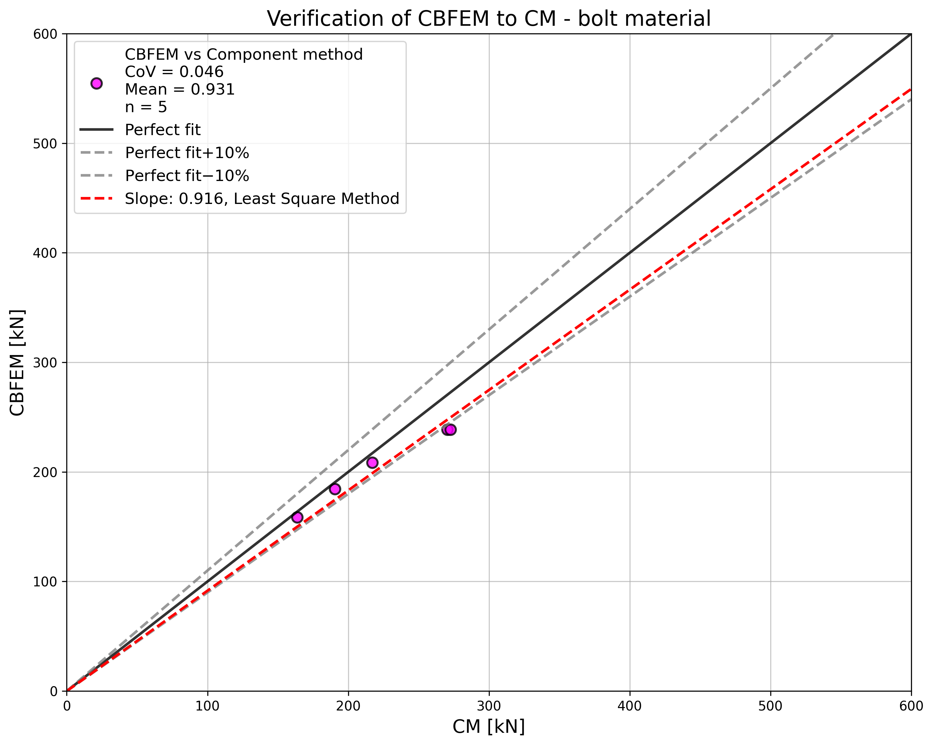
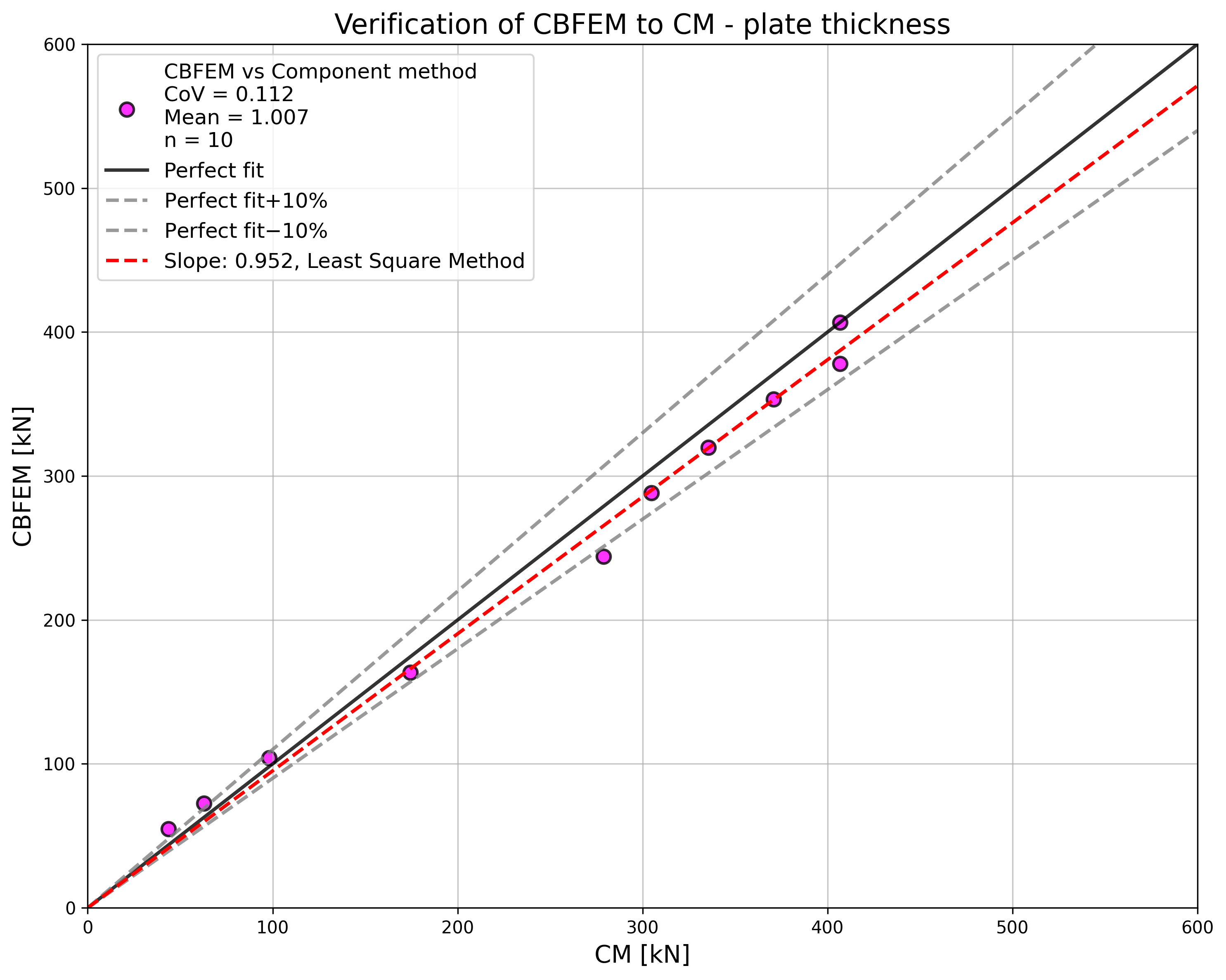
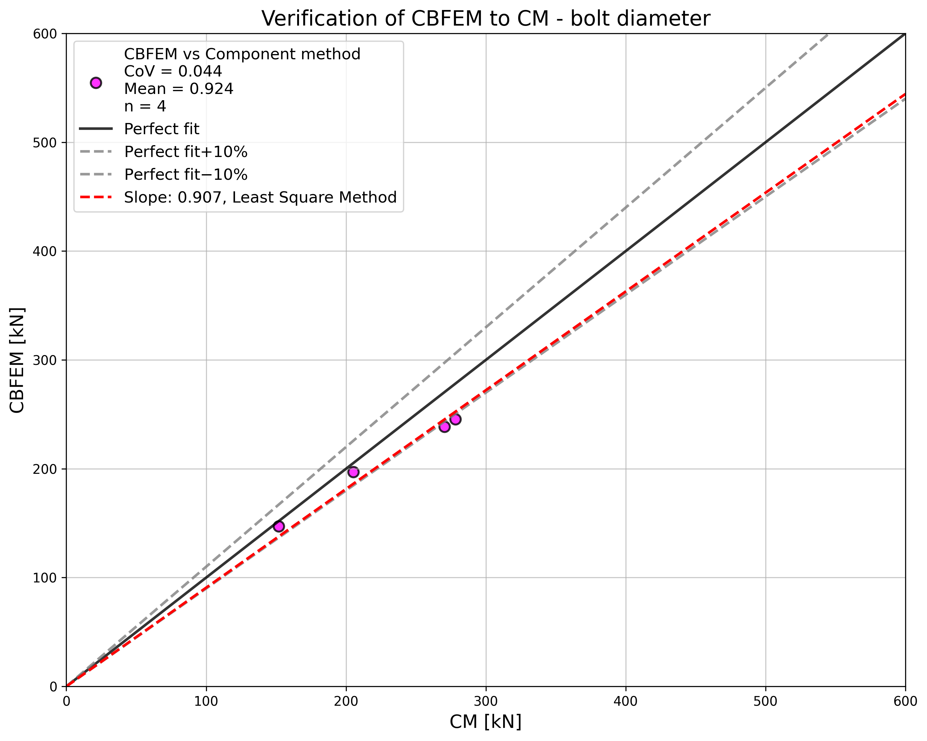
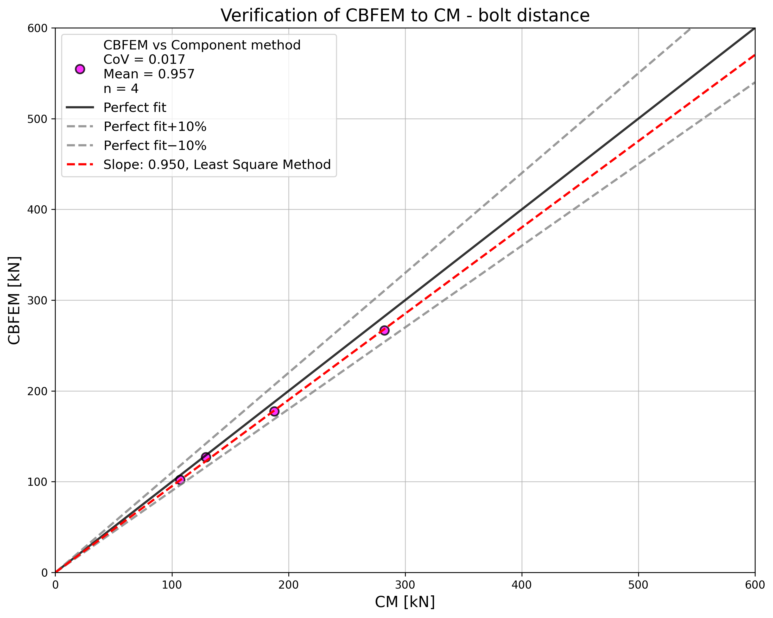
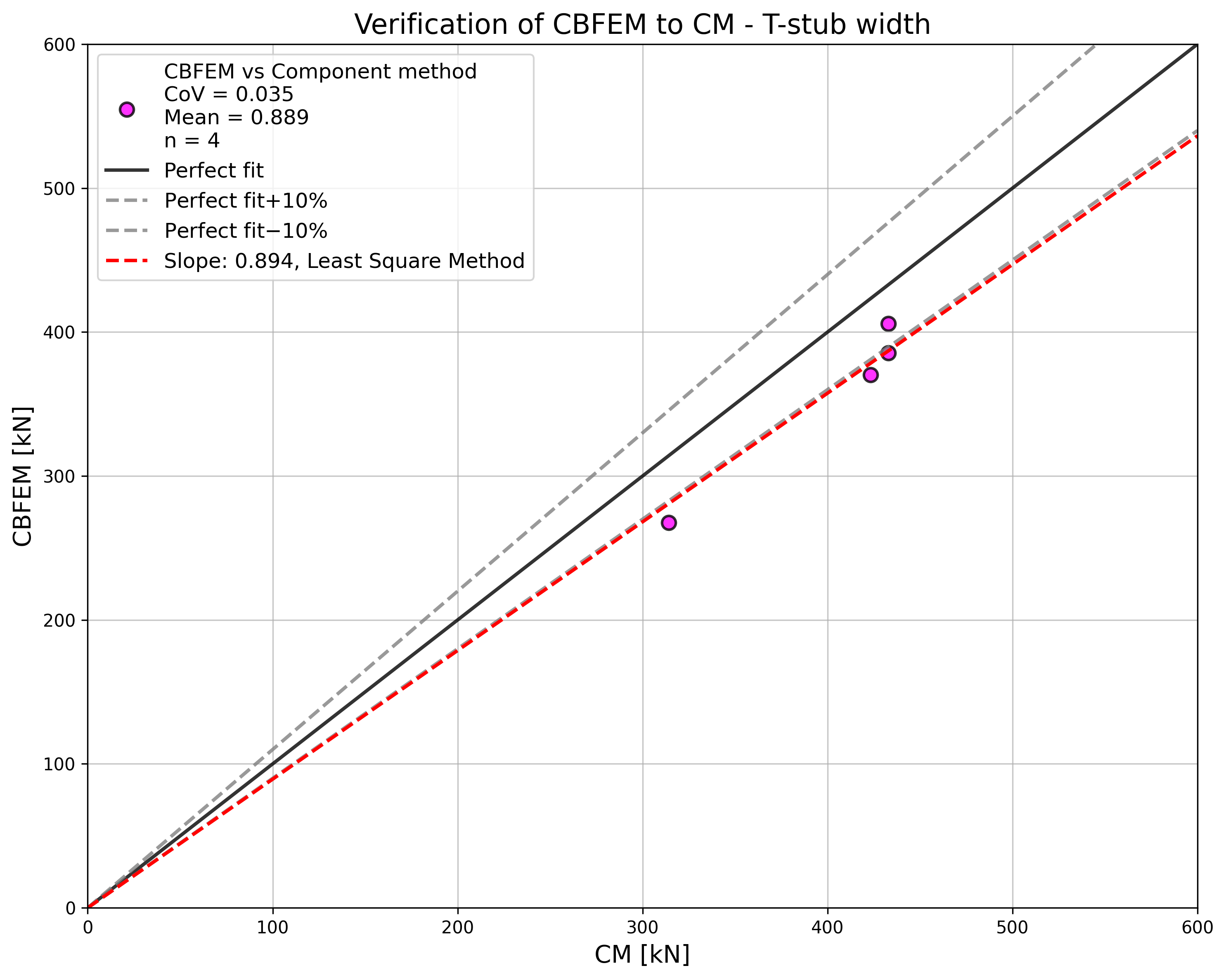
\[ \textsf{\textit{\footnotesize{Fig. 5.1.10 Summary of verification of CBFEM to CM}}}\]

Exemplu de referință

Date de intrare

T-stub, a se vedea Fig. 5.1.11

• Oțel S235
• Grosimea tălpii t_f = 20 mm
• Grosimea inimii t_w = 20 mm
• Lățimea tălpii b_f = 300 mm
• Lungimea b = 100 mm
• Sudură de colț dublă a_w = 10 mm

Șuruburi

• 2 × M24 8.8
• Distanța dintre șuruburi w = 165 mm

Configurare cod – Model și plasă

• Numărul de elemente pe cel mai mare element sau talpă 16

Rezultate

• Rezistența de calcul la întindere F_T,Rd = 164 kN
• Mod de cedare – plastifierea completă a tălpii cu deformația maximă de 5 %
• Gradul de utilizare al șuruburilor 86,4 %
• Gradul de utilizare al sudurilor 45,7 %

\[ \textsf{\textit{\footnotesize{Fig. 5.1.11 Benchmark example for the T-stub}}}\]

Referințe

EN 1993-1-5, Eurocode 3, Design of steel structures – Part 1-5: Plated Structural Elements, CEN, Brussels, 2005.

EN 1993-1-8, Eurocode 3, Design of steel structures – Part 1-8: Design of joints, CEN, Brussels, 2005.

Beg D., Zupančič E., Vayas I. On the rotation capacity of moment connections, Journal of Constructional Steel Research, 60 (3–5), 2004, 601–620.

Gödrich L., Wald F., Sokol Z. To Advanced modelling of end plate joints, Connection and Joints in Steel and Composite Structures, Rzeszow, 2013.

Gödrich L., Wald F., Kabeláč J., Kuříková M. Design finite element model of a bolted T-stub connection component, Journal of Constructional Steel Research. 2019, (157), 198-206.

Wu Z., Zhang S., Jiang S. Simulation of tensile bolts in finite element modelling of semi-rigid beam-to-column connections, International Journal of Steel Structures 12 (3), 2012, 339-350.

Îmbinare cu șuruburi - Eclise la forfecare

Descriere

Acest studiu este axat pe verificarea metodei elementelor finite bazate pe componente (CBFEM) pentru rezistența îmbinării cu eclise duble simetrice cu șuruburi față de un model analitic (MA).

Model analitic

Rezistența șuruburilor la forfecare și rezistența plăcilor la presiune pe gaură sunt calculate conform Tab. 3.4 din capitolul 3.6.1 din EN 1993-1-8:2005. Pentru îmbinări lungi, se ia în considerare factorul de reducere conform pct. 3.8. Rezistența de calcul a elementelor îmbinate cu reduceri pentru găurile dispozitivelor de fixare este luată în considerare conform pct. 3.10.

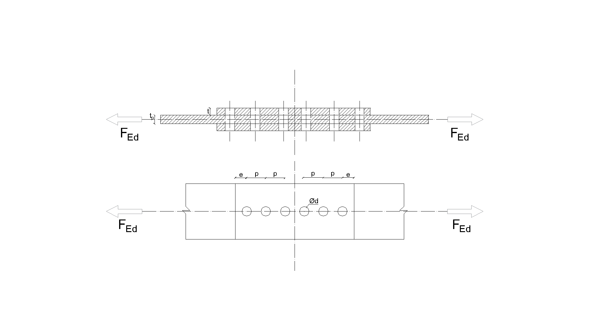
\[ \textsf{\textit{\footnotesize{ Drawing 5.2.1 Joint geometry and dimensions}}}\]

Verificarea rezistenței

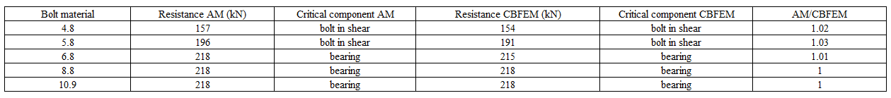
Rezistențele de calcul calculate prin CBFEM au fost comparate cu rezultatele modelului analitic (MA). Rezultatele sunt rezumate în Tab. 5.2.1. Parametrii sunt materialul șuruburilor, grosimea eclisei, diametrul șuruburilor și distanțele dintre șuruburi, a se vedea Fig. 5.2.1 până la 5.2.4.

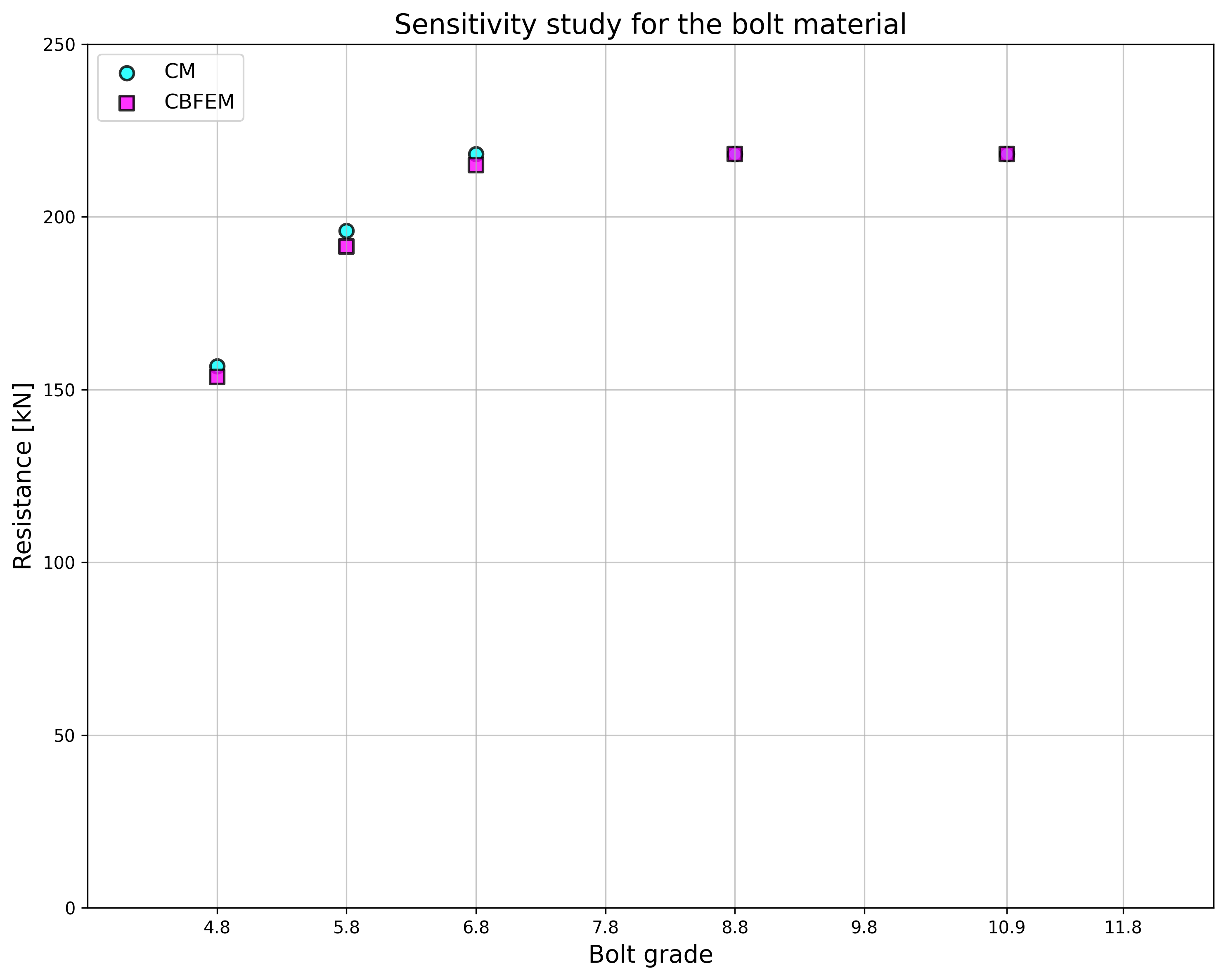
\[ \textsf{\textit{\footnotesize{Fig. 5.2.1 Sensitivity study for the bolt material}}}\]

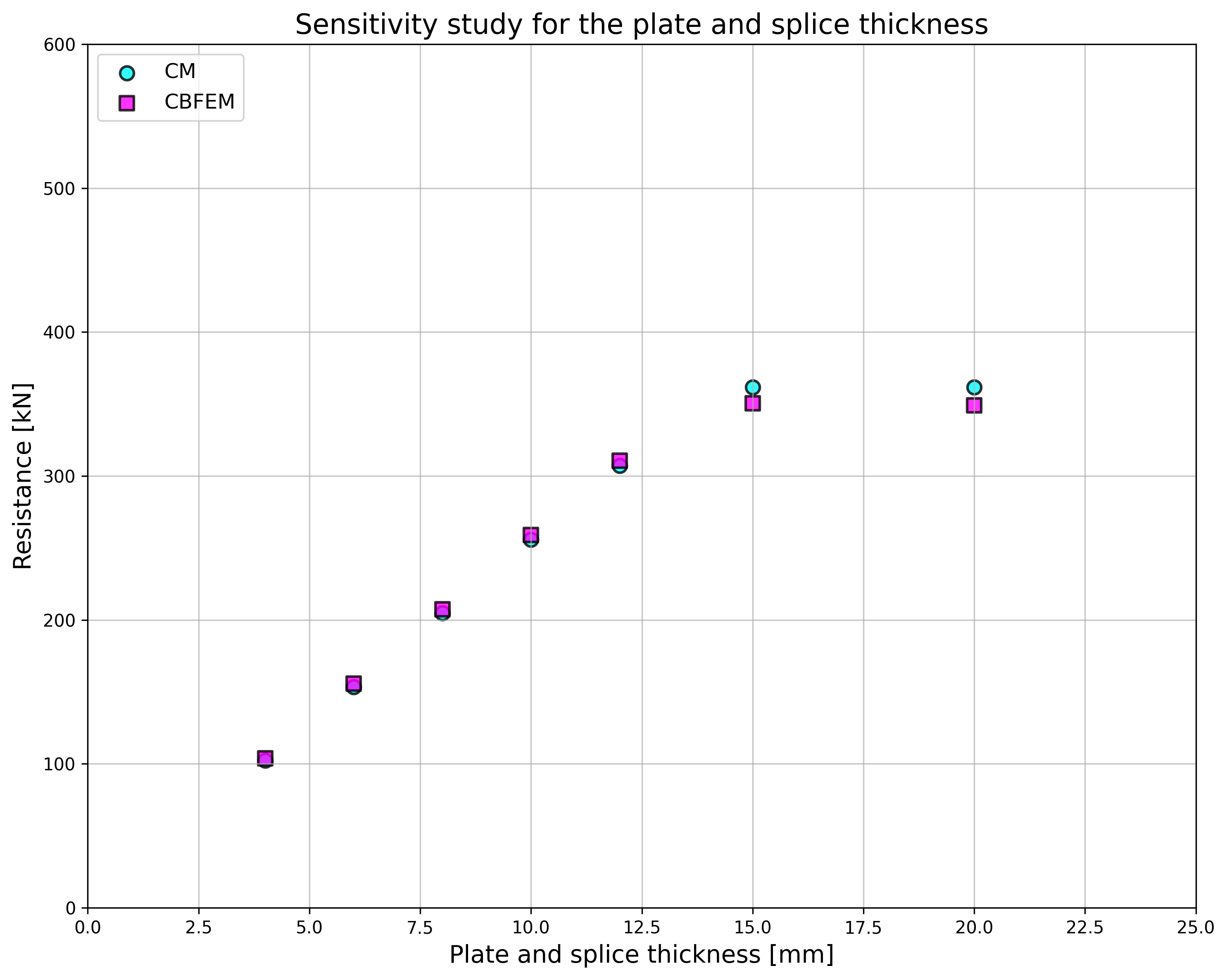
\[ \textsf{\textit{\footnotesize{Fig. 5.2.2 Sensitivity study for the splice thickness}}}\]

Tab. 5.2.1 Studiu de sensibilitate al rezistenței

Descrierea nodului: eclisat 150/10mm, șuruburi 2×M20 la distanțele p =70, e₁=50, plăci 2×150/6mm, oțel S235

Descrierea nodului: înălțimea eclisei 200mm, șuruburi 3×M16 8,8 la distanțele p = 55mm e₁ = 40mm, plăci 2×200/t mm, oțel S235

Descrierea nodului: eclisat 120/10mm, șuruburi 2×MX 8,8, plăci 2×120/10 mm, oțel S235

Descrierea nodului: Eclisat 200/6 mm, șuruburi 3×M16 8,8, plăci 2×200/6mm, oțel S235

\[ \textsf{\textit{\footnotesize{Fig. 5.2.3 Sensitivity study for the bolt diameter}}}\]

\[ \textsf{\textit{\footnotesize{Fig. 5.2.4 Sensitivity study for the distance of bolts}}}\]

Rezultatele studiilor de sensibilitate sunt rezumate în graficul din Fig. 5.2.5. Rezultatele arată că diferențele dintre cele două metode de calcul sunt sub 5 %. Modelul analitic oferă în general o rezistență mai mare.

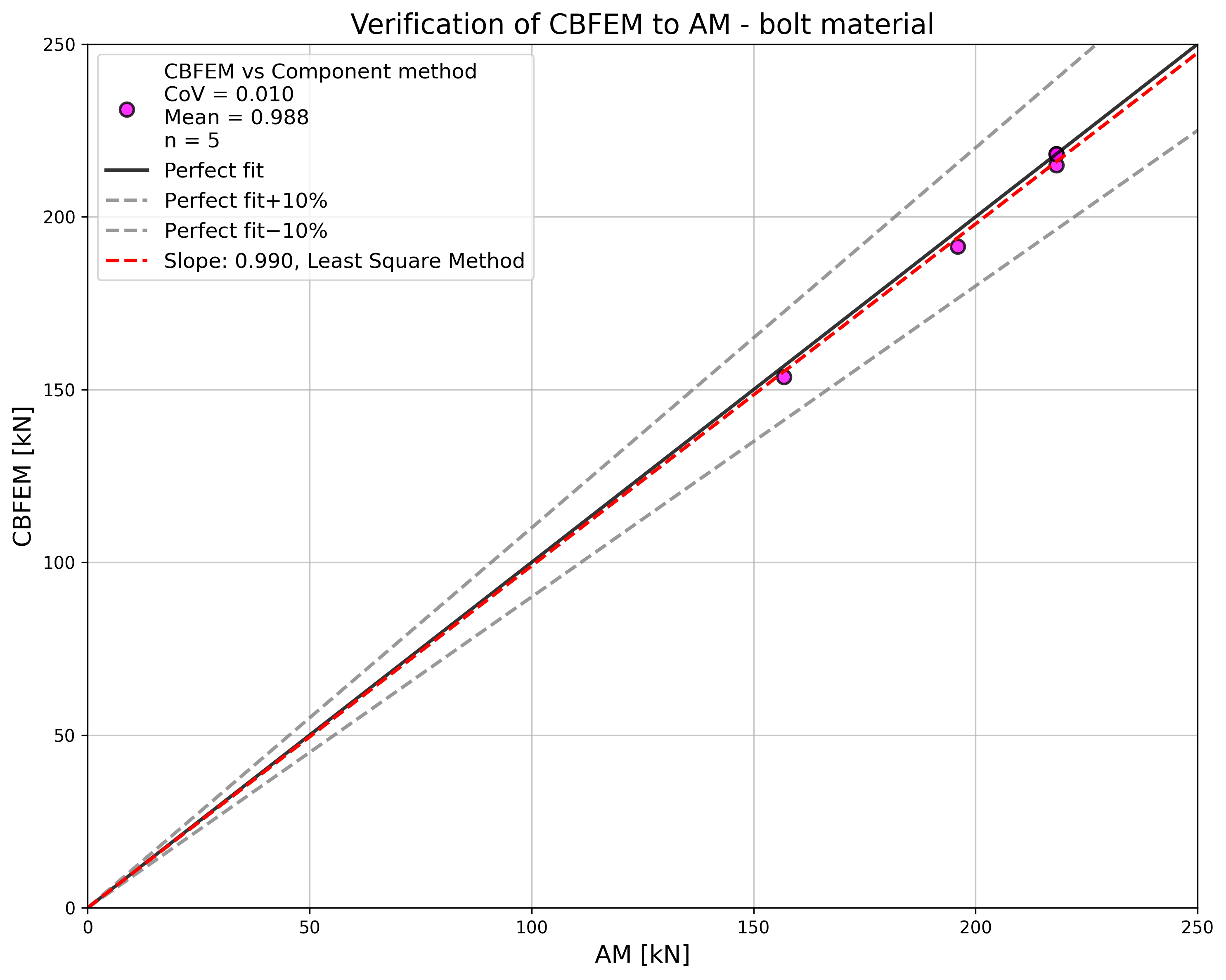
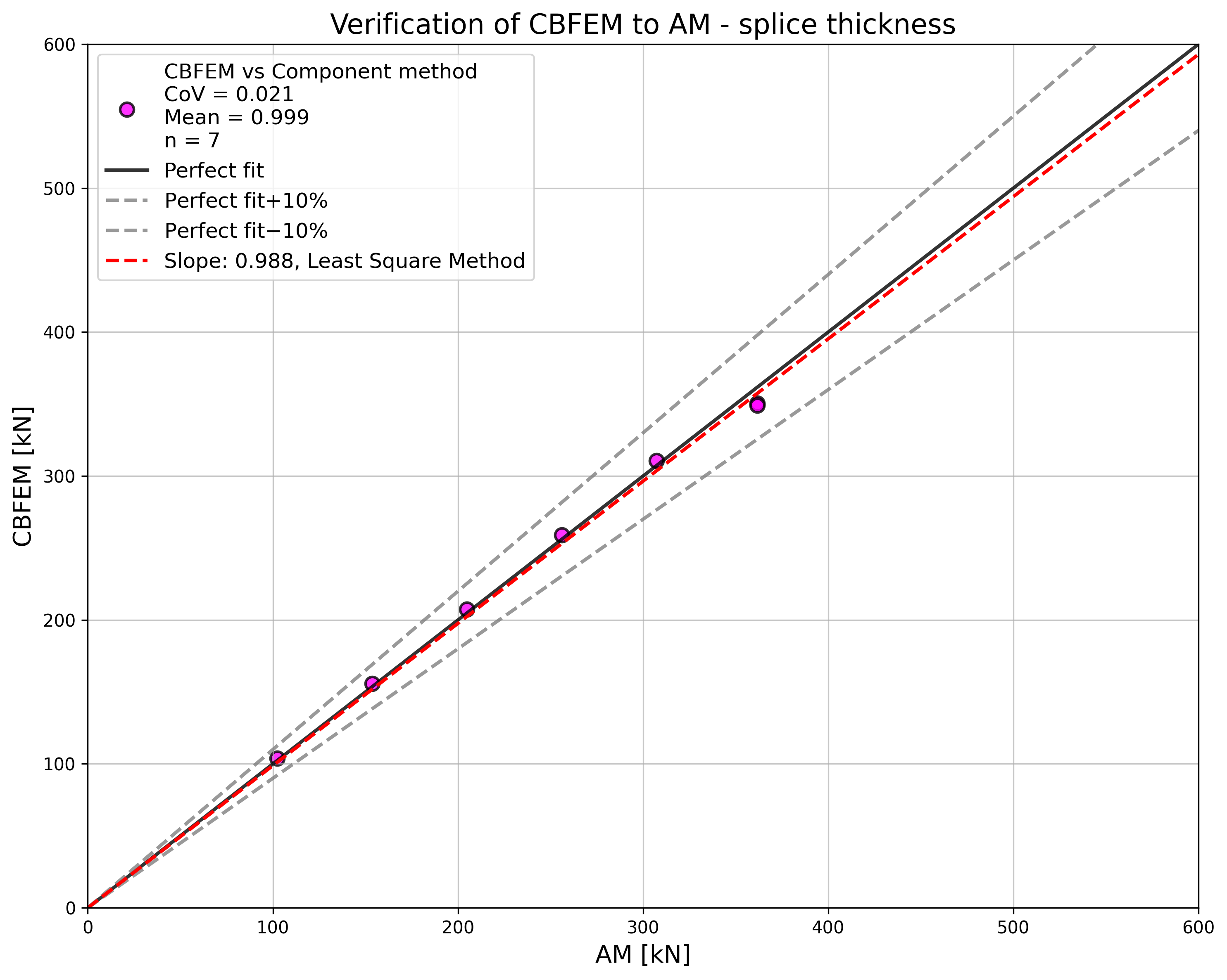
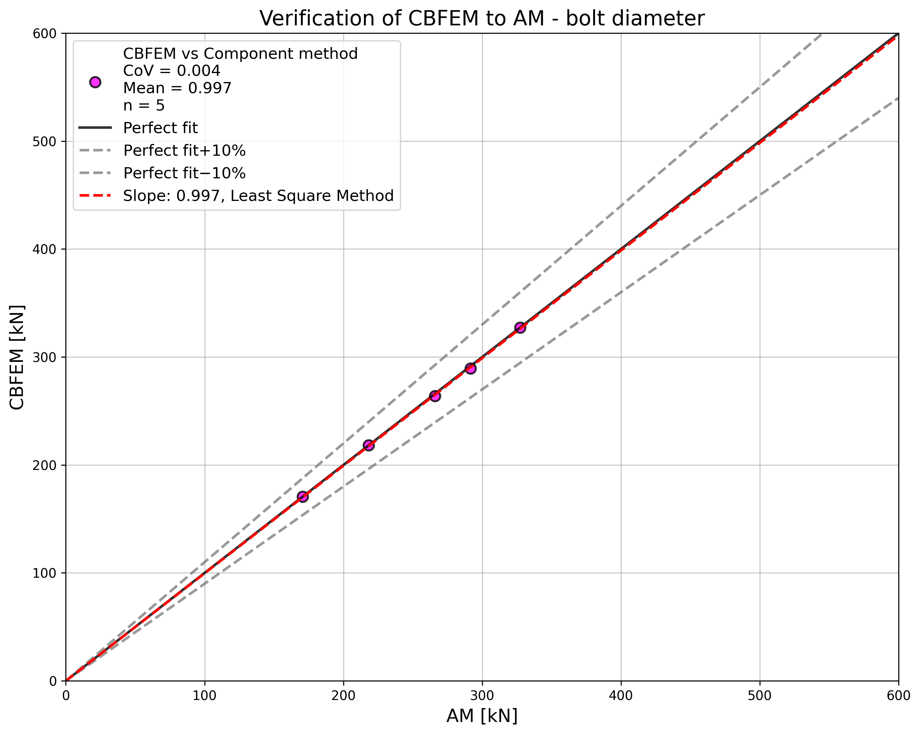
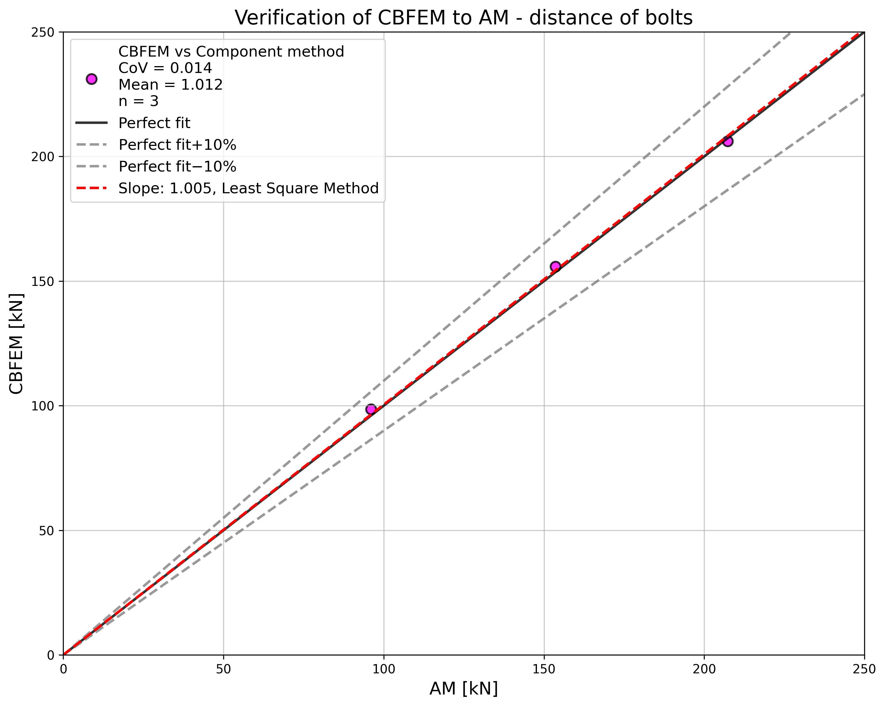
\[ \textsf{\textit{\footnotesize{Fig. 5.2.5 Verification of CBFEM to AM for the symmetrical double splice connection}}}\]

Exemplu de referință

Date de intrare

Element îmbinat

• Oțel S235
• Eclisat 200/10 mm

Conectori

Șuruburi

• 3 × M16 8.8
• Distanțe e₁ = 40 mm, p = 55 mm

2 x eclisat

• Oțel S235
• Placă 380×200×10

Rezultate

• Rezistența de calcul F_Rd = 258 kN
• Determinantă este presiunea pe gaură a eclisei îmbinate

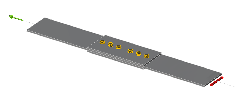
\[ \textsf{\textit{\footnotesize{Fig. 5.2.6 Benchmark example of the bolted splices in shear}}}\]

Îmbinare cu placă de capăt pe axa slabă

Descriere

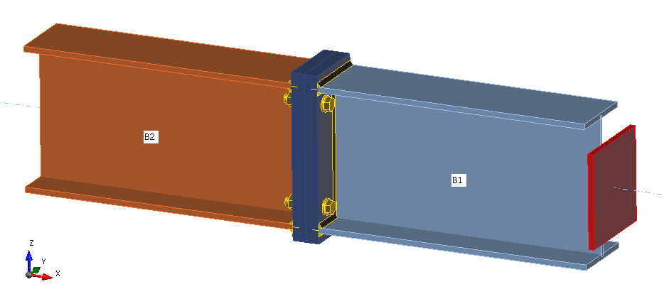
Modelul CBFEM (Metoda Elementelor Finite bazată pe componente) al îmbinării grindă-stâlp este verificat prin Metoda Componentelor (CM). Placa de capăt extinsă cu trei rânduri de șuruburi este conectată la inima stâlpului și încărcată cu moment încovoietor; a se vedea Fig. 5.3.1.

\[ \textsf{\textit{\footnotesize{Fig. 5.3.1 Joint geometry - all dimensions in mm}}}\]

Model analitic

Cele trei componente care guvernează comportamentul sunt: placa de capăt la încovoiere, talpa grinzii la întindere și la compresiune, și inima stâlpului la încovoiere. Placa de capăt și talpa grinzii la întindere și la compresiune sunt proiectate conform EN 1993-1-8:2005. Comportamentul inimii stâlpului la încovoiere este estimat conform (Steenhuis et al. 1998). Rezultatele experimentelor privind îmbinările grindă-stâlp pe axa slabă, de ex. (Lima et al. 2009), arată o bună predicție a acestui tip de îmbinare încărcată în planul grinzii conectate.

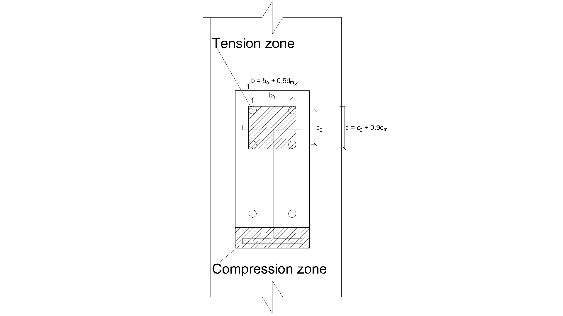
\[ \textsf{\textit{\footnotesize{Fig. 5.3.2 Definition of the tension zone}}}\]

\[F_\mathrm{{local.Rd }}=\min \left(F_\mathrm{{punch.Rd }} ; F_\mathrm{{comb.Rd }}\right)\]

\[F_\mathrm{ {punch.Rd }}  = n \cdot \pi\cdot d_\mathrm{m}  \cdot t_\mathrm{w c} \cdot f_\mathrm{y} /\left(\sqrt{3} \cdot \gamma_\mathrm{M 0}\right) \quad \text{bolted end plate }\] 

\[b = b_0 + 0.9 \cdot d_\mathrm{m}\]

\[c = c_0 + 0.9 \cdot d_\mathrm{m}\]

\[a = L - b\]

\[k= 1 \quad \text{ if }\quad(b+c) / L>0.5\]

\[k=0.7+0.6(b+c) / L \quad \text{ if }\quad(b+c) / L \leq 0.5\]

\[b_\mathrm{m}=L\left[1-0.82 \frac{t_\mathrm{w c}^2}{c^2}\left(1+\sqrt{1+2.8 \frac{c^2}{t_\mathrm{w c} L}}\right)^2\right], \quad \text{ but } \quad b_\mathrm{m} \geq 0\]

\[x_0=L\cdot\left[\left(\frac{t_\mathrm{w c}}{L}\right)^{\frac{2}{3}}+0.23 \frac{c}{L}\left(\frac{t_\mathrm{w c}}{L}\right)^{\frac{1}{3}}\right] \cdot\left(\frac{b-b_\mathrm{m}}{L-b_\mathrm{m}}\right)\]

\[x = 0 \quad b \leq b_\mathrm{m}\]

\[x=-a+\sqrt{a^2-1.5 a c+\frac{\sqrt{3}}{2} t_\mathrm{w c}\left[\pi \sqrt{L\left(a+x_0\right)}+4 c\right]} \quad \text{ if }\quad b>b_\mathrm{m}\]

\[F_\mathrm{c o m b . R d}=k\cdot t_\mathrm{w c}^2 \cdot f_\mathrm{y}\left[\frac{\pi \sqrt{L(a+x)}+2 c}{a+x}+\frac{1.5 c x+x^2}{\sqrt{3} t_\mathrm{w c}(a+x)}\right] / \gamma_\mathrm{M 0}\]

\[\rho = 1 \quad \text{ if }\quad z / (L-b) \leq 1\]
\[\rho = z / (L-b) \quad \text{ if }\quad 1<z / (L-b) \leq 10\]

\[F_\mathrm{g l o b a l . R d}=\frac{F_\mathrm{c o m b . R d}}{2}+\frac{t_\mathrm{w c}^2 f_\mathrm{y}}{4}\left(\frac{2 b}{z}+\pi+2 \rho\right) / \gamma_\mathrm{M 0}\]

\[F_\mathrm{Rd} = \min \left(F_\mathrm{{local.Rd }} ; F_\mathrm{g l o b a l . R d}\right)\]

\[M_\mathrm{Rd} = z \cdot F_\mathrm{Rd}\]

Unde:

• \(t_\mathrm{w c} \quad\) este grosimea inimii stâlpului
• \(f_\mathrm{y} \quad\) este limita de curgere a inimii stâlpului
• \(\gamma_{\mathrm{M} 0}\) este factorul parțial de siguranță al oțelului
• \(\gamma_{\mathrm{M} 0}\) este factorul parțial de siguranță al oțelului
• \(n\) numărul de rânduri de șuruburi la întindere
• \(d_\mathrm{m}\) diametrul diagonal al capului șurubului
• \(b_0\) distanța orizontală dintre șuruburi 
• \(c_0\) distanța verticală dintre șuruburi
• \(z\) brațul de pârghie al îmbinării
• \(F_\mathrm{ {punch.Rd }} \quad\) este rezistența la forfecare prin poansonare
• \(F_\mathrm{ {comb.Rd }} \quad\) este rezistența la poansonare combinată, forfecare și încovoiere

Model numeric

Evaluarea se bazează pe deformația maximă specificată conform EN 1993-1-5:2006 prin valoarea de 5 %. Informații detaliate despre modelul CBFEM sunt rezumate în Capitolul 3.

Verificarea rezistenței

Studiul de sensibilitate al rezistenței îmbinării a fost realizat pentru secțiunile transversale ale stâlpului. Geometria îmbinării este prezentată în Fig. 5.3.1. În Tab. 5.3.1 și în Fig. 5.3.3 sunt rezumate rezultatele calculelor în cazul măririi plăcii de capăt P18 în raport cu secțiunea stâlpului.

Tab. 5.3.1 Rezultatele predicției îmbinării cu placă de capăt pe axa slabă pentru diferite grinzi de acoperiș

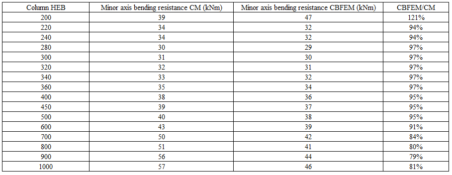
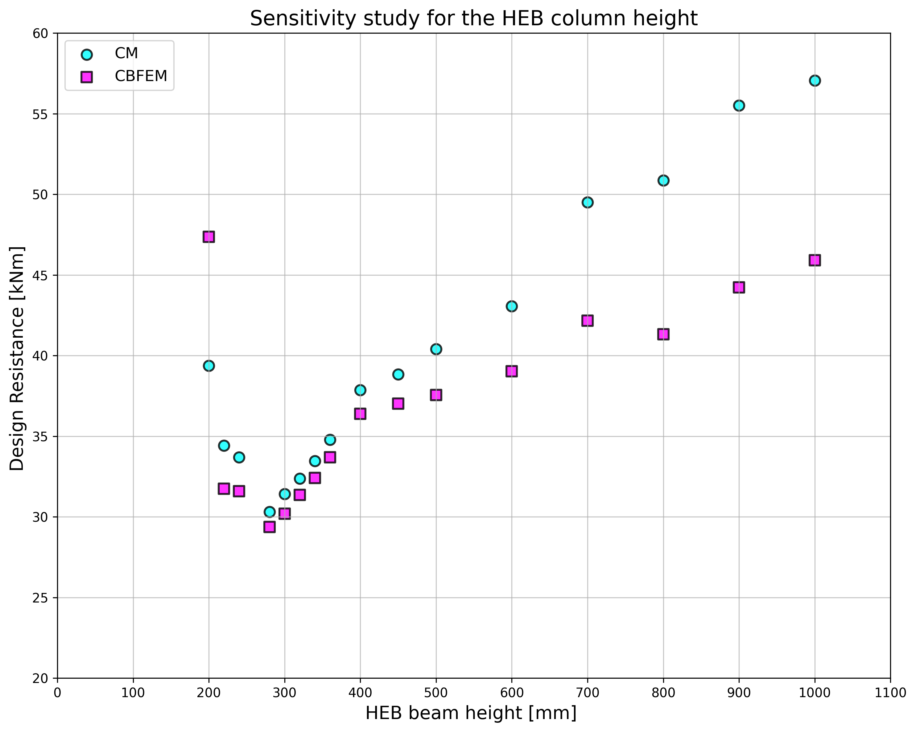
\[ \textsf{\textit{\footnotesize{Fig. 5.3.3 Comparison resistance of end plate minor axis connection predicted by CBFEM and CM}}}\]

Comportament global

Comportamentul global este prezentat pe curba forță-deformație. Grinda IPE 240 este conectată la stâlpul HEB 300 cu șase șuruburi M16 8.8. Geometria plăcii de capăt este prezentată în Fig. 5.3.1 și în Tab. 5.3.1. Compararea rezultatelor ambelor metode este prezentată în Fig. 5.3.4 și în Tab. 5.3.2. Ambele metode estimează o rezistență de calcul similară. CBFEM oferă în general o rigiditate inițială mai mică comparativ cu CM. 

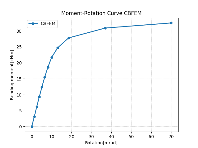
\[ \textsf{\textit{\footnotesize{Fig. 5.3.4 Prediction of behavior of end plate minor axis connection on moment rotational curve CBFEM}}}\]

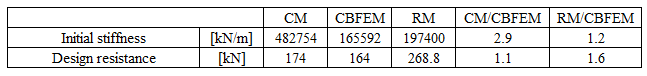
Tab. 5.3.2 Caracteristici principale pentru comportamentul global

		CM	CBFEM	CM/CBFEM
Rigiditate inițială	[kNm/rad]	16130	2232	7.23
Rezistență de calcul	[kNm]	31	30	1,03

Rezultatele studiilor sunt rezumate în graficul care compară rezistențele obținute prin CBFEM și metoda componentelor; a se vedea Fig. 5.3.5. Rezultatele arată că diferența dintre metode este de până la 14 %. CBFEM estimează în toate cazurile o rezistență mai mică comparativ cu CM, care se bazează pe simplificările din (Steenhuis et al. 1998). Rezultate similare pot fi observate în lucrarea (Wang și Wang, 2012).

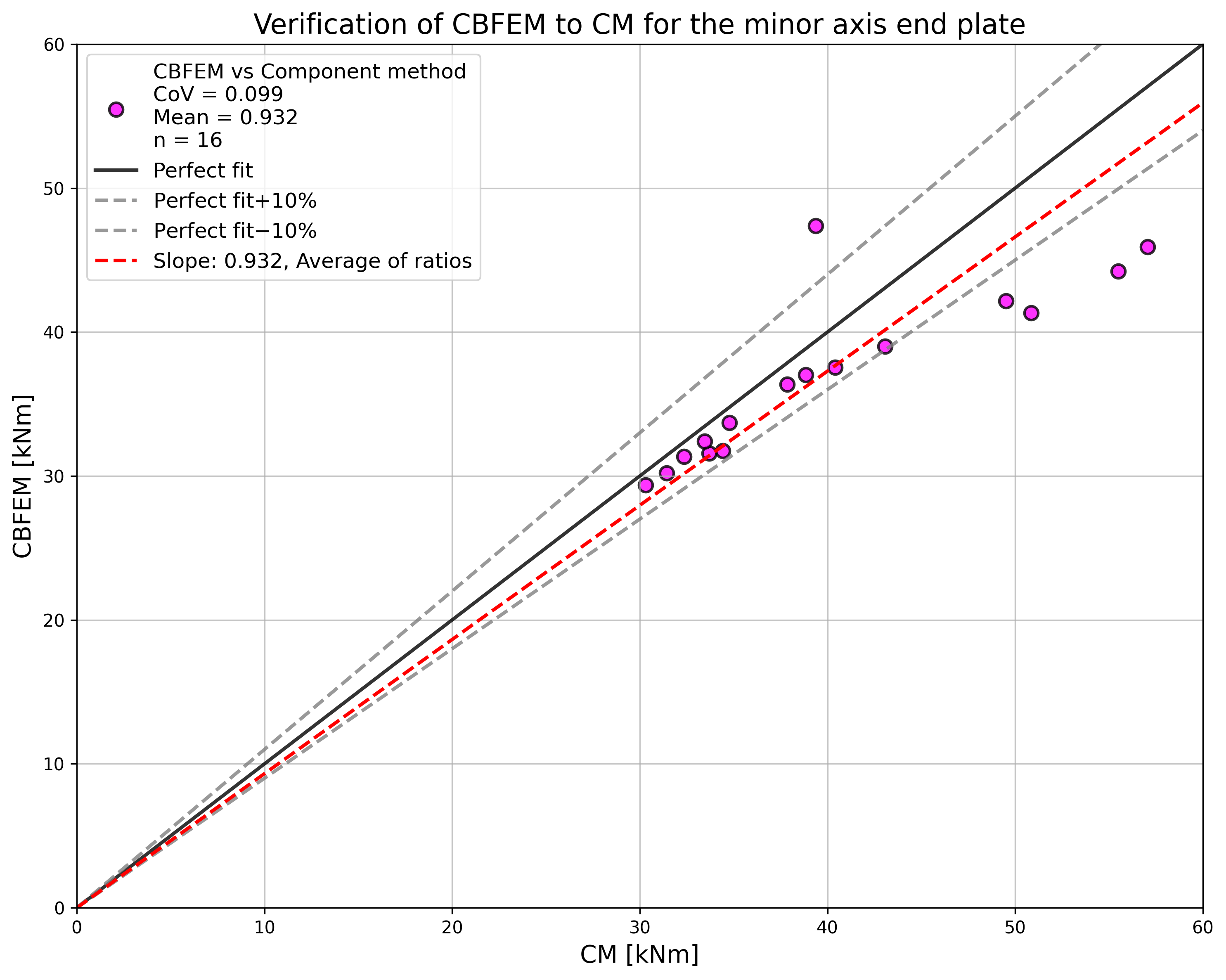
\[ \textsf{\textit{\footnotesize{Fig. 5.3.5 Summary of verification of CBFEM to CM for the end plate minor axis connection}}}\]

Exemplu de referință

Cazul de referință este pregătit pentru îmbinarea cu placă de capăt pe axa slabă conform Fig. 5.3.1 cu geometria modificată rezumată mai jos.

Date de intrare

• Oțel S235
• Stâlp HEB 300
• Grindă IPE 240
• Șuruburi 6×M16 8.8
• Grosimea sudurilor 5 mm
• Grosimea plăcii de capăt t_p = 18 mm

Rezultate

• Rezistența de calcul la încovoiere M_Rd = 30 kNm
• Componenta determinantă – inima stâlpului la încovoiere

Referințe

EN 1993-1-5, Eurocode 3, Design of steel structures – Part 1-5: Plated Structural Elements, CEN, Brussels, 2005.

Steenhuis M., Jaspart J. P., Gomes F., Leino T. Application of the component method to steel joints, in Control of the Semi-rigid Behaviour of Civil Engineering Structural Connections Conference, COST C1, Liege, Belgium, 1998, 125-143.

Wang Z., Wang T. Experiment and finite element analysis for the end plate minor axis connection of semi-rigid steel frames, Tumu Gongcheng Xuebao/China Civil Engineering Journal, 45 (8), 2012, 83-89.

Îmbinare cu șuruburi - Interacțiunea dintre forfecare și întindere

Descriere

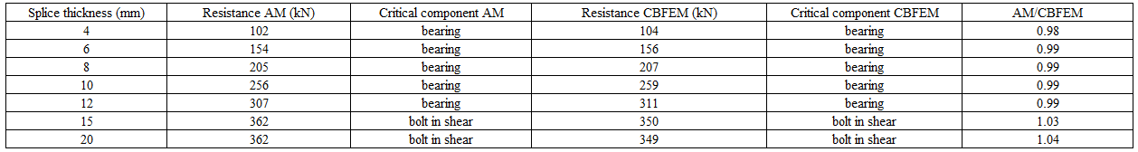
Obiectivul acestui capitol este verificarea metodei cu elemente finite bazate pe componente (CBFEM) pentru interacțiunea dintre forfecare și întindere într-un șurub față de un model analitic (AM). Pentru verificare a fost selectată o îmbinare grindă-grindă cu plăci de capăt și două rânduri de șuruburi; a se vedea Fig. 5.5.1. Rigiditatea la încovoiere a îmbinării este suficient de mare pentru a fi clasificată ca rigidă.

\[ \textsf{\textit{\footnotesize{Fig. 5.5.1 Joint arrangement of bolted beam-to-beam joint}}}\]

Model analitic

Rezistența șurubului la interacțiunea dintre forfecare și întindere este proiectată conform Tab. 3.4 din capitolul 3.6.1 din EN 1993-1-8:2005. Se utilizează o relație bilineară. Geometria și dimensiunile plăcii de capăt ale îmbinării sunt selectate pentru a limita rezistența de calcul a îmbinării prin cedarea șurubului. Rezistența de calcul a tronsonului T echivalent la întindere este modelată conform Tab. 6.2 din capitolul 6.2.4 din EN 1993‑1‑8:2005.

Verificarea rezistenței

Parametrii modelului sunt diametrul șurubului și dimensiunea grinzii; a se vedea Fig. 5.5.2 până la 5.5.5. Dimensiunile plăcii de capăt și distanțele dintre șuruburi sunt modificate pentru a limita rezistența îmbinării prin cedarea șurubului. Rezistența la forfecare și la încovoiere a îmbinării este comparată la încărcarea corespunzătoare cedării șurubului. Rezultatele sunt rezumate în Tab. 5.5.1 și 5.5.2.

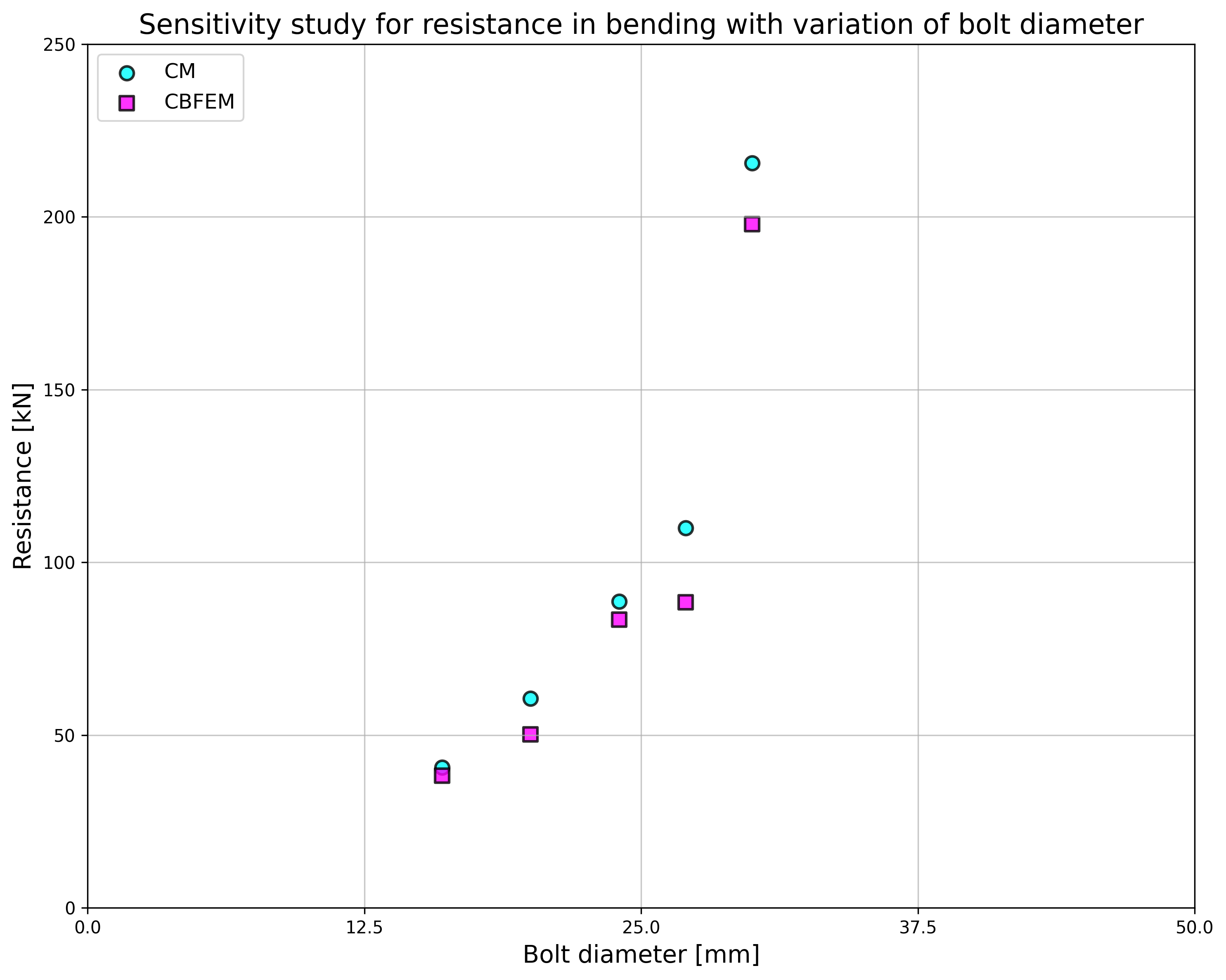
\[ \textsf{\textit{\footnotesize{Fig. 5.5.2 Sensitivity study for resistance in bending with variation of bolt diameter}}}\]

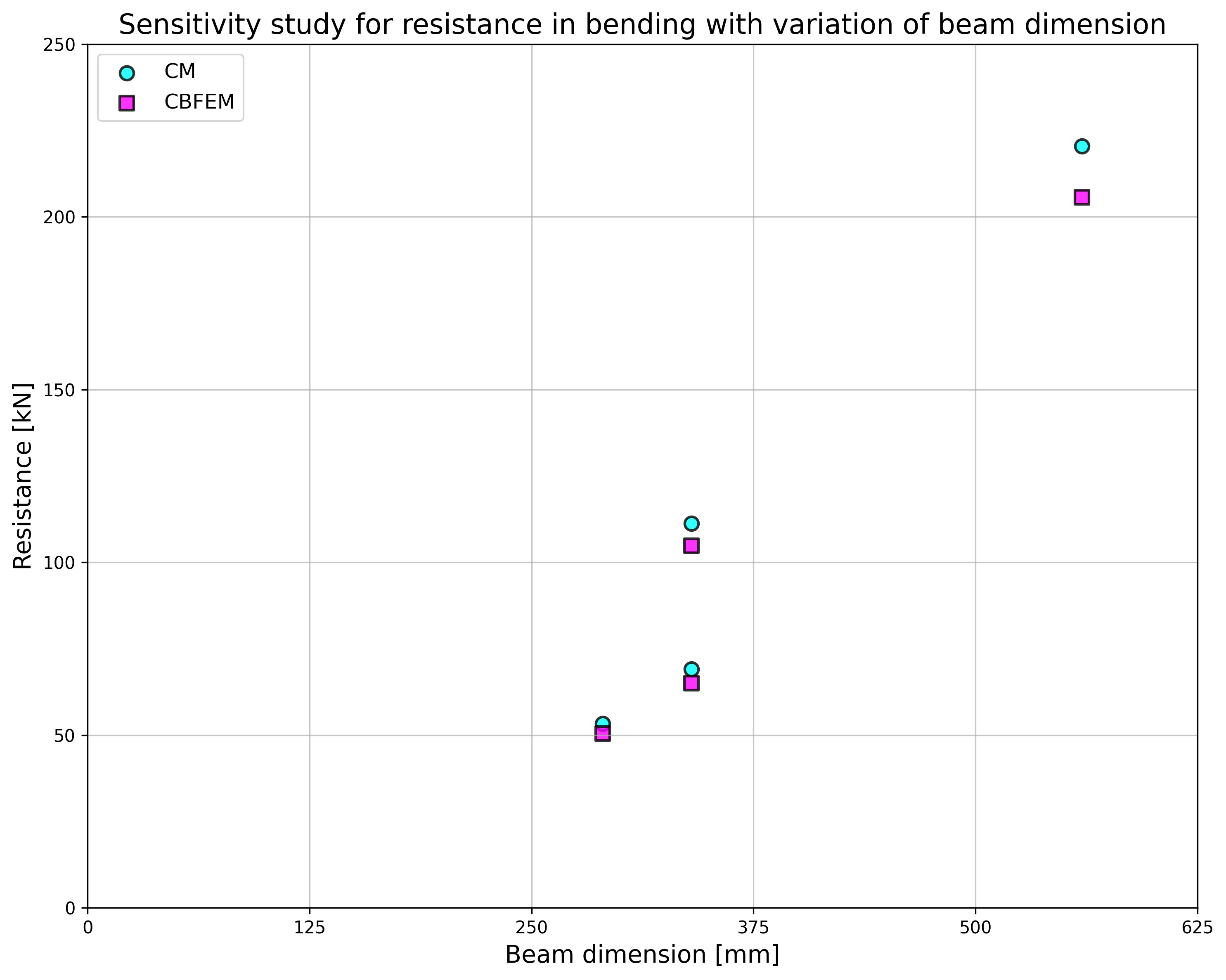
\[ \textsf{\textit{\footnotesize{Fig. 5.5.3 Sensitivity study for resistance in bending with variation of beam dimension}}}\]

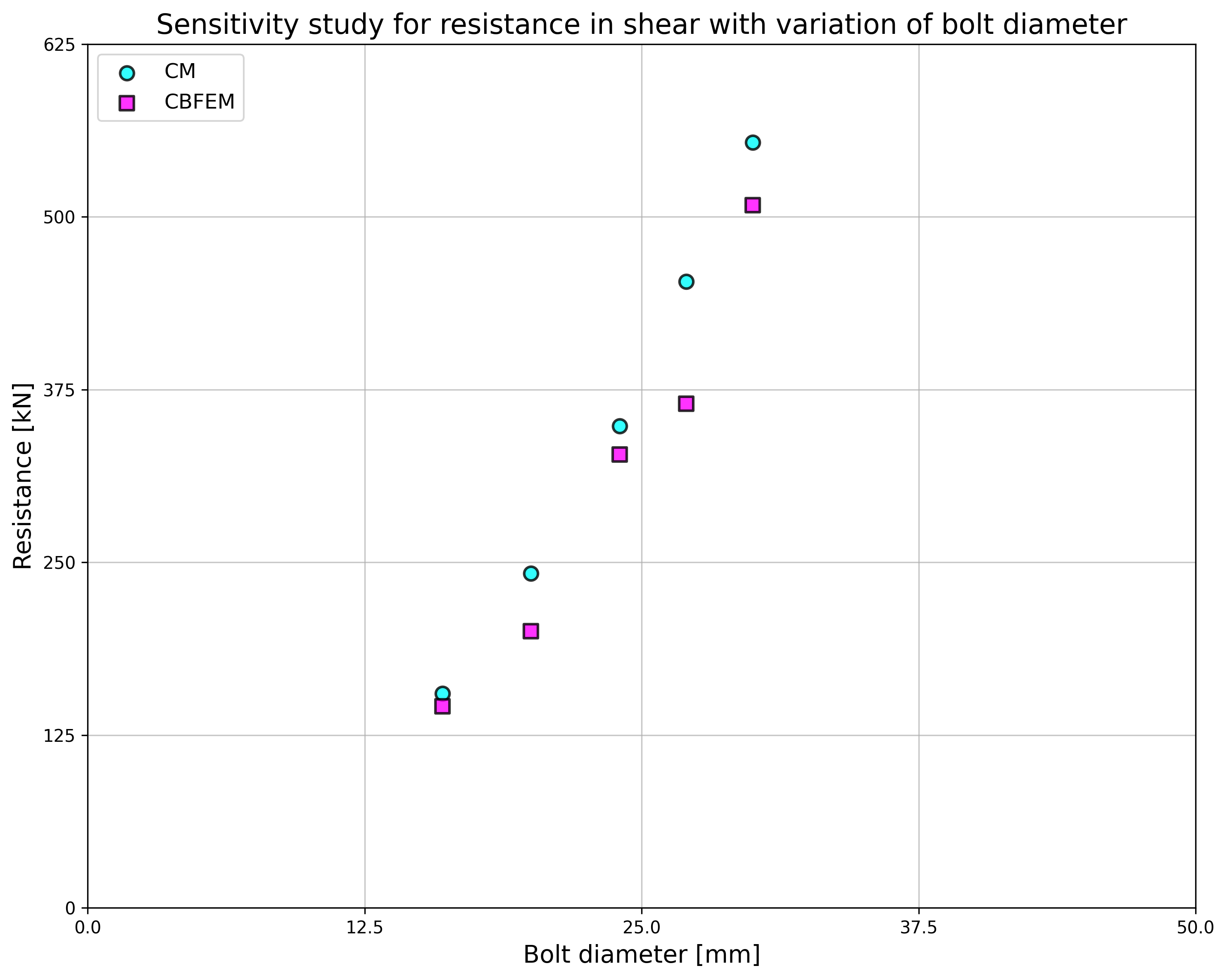
\[ \textsf{\textit{\footnotesize{Fig. 5.5.4 Sensitivity study for resistance in shear with variation of bolt diameter}}}\]

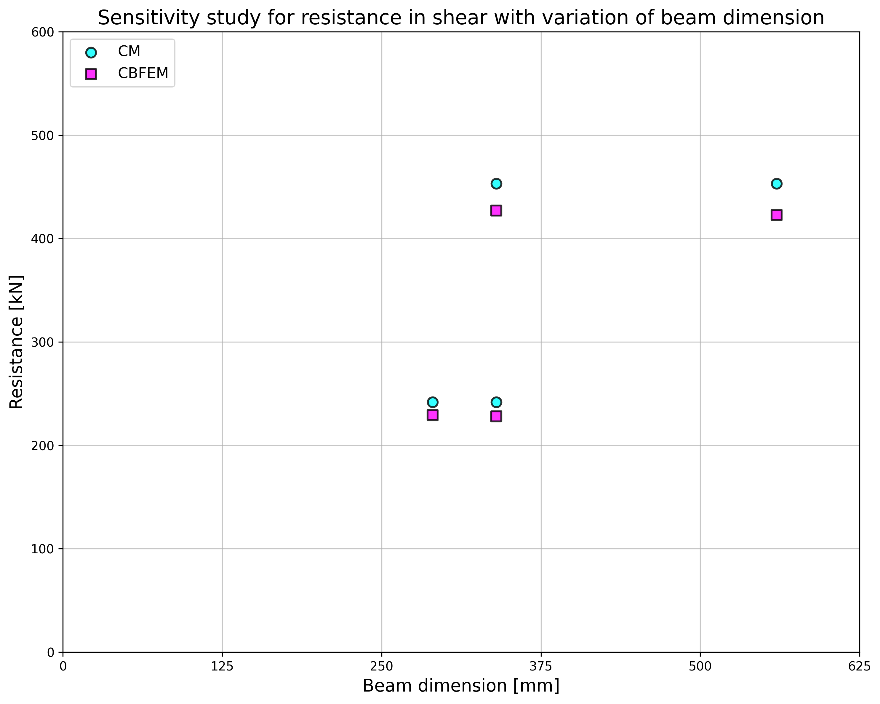
\[ \textsf{\textit{\footnotesize{Fig. 5.5.5 Sensitivity study for resistance in shear with variation of beam dimension}}}\]

Tab. 5.5.1 Studiu de sensibilitate pentru rezistență cu variația diametrului șurubului

Parametru			AM		CBFEM		AM/CBFEM
Grindă;             placă de capăt	Diametru	Distanțe	MRd [kNm]	VRd [kN]	MRd [kNm]	VRd [kN]	MRd	VRd
IPE270; tp = 30mm; 150×310mm	M16/8.8	e1 = 60 mm; p1 = 190 mm; w = 90 mm	41	155	38	146	1,06	1,06
	M20/8.8	e1 = 70 mm; p1 = 170 mm; w = 90 mm	61	242	50	200	1,21	1,21
HEA300; tp = 40mm; 300×330mm	M24/8.8	e1 = 85 mm; p1 = 160 mm; w = 150 mm	89	349	83	328	1,06	1,06
	M27/8.8	e1 = 95 mm; p1 = 140 mm; w = 150 mm	110	453	89	365	1,24	1,24
HEA500; tp = 40mm; 330×520mm	M30/8.8	e1 = 160 mm; p1 = 200 mm; w = 150 mm	216	554	198	509	1,09	1,09

Tab. 5.5.2 Studiu de sensibilitate pentru rezistență cu variația dimensiunii grinzii

Parametru			AM	AM	CBFEM	CBFEM	AM/CBFEM	AM/CBFEM
Grindă; placă de inimă	Diametru	Distanțe	MRd [kNm]	VRd [kN]	MRd [kNm]	VRd [kN]	MRd	VRd
HEA260; tp = 25mm; 260×290mm	M20/8.8	e1 = 75 mm; p1 = 140 mm; w = 130 mm	53	242	50	229	1,06	1,06
IPE300; tp = 30mm; 150×340mm	M20/8.8	e1 = 70 mm; p1 = 200 mm; w = 90 mm	69	242	65	228	1,06	1,06
HEB300; tp = 40mm; 300×340mm	M27/8.8	e1 = 100 mm; p1 = 140 mm; w = 150 mm	111	453	105	427	1,06	1,06
IPE500; tp = 45mm; 220×560mm	M27/8.8	e1 = 105 mm; p1 = 350 mm; w = 120 mm	220	453	206	423	1,07	1,07

\[ \textsf{\textit{\footnotesize{Drawing 5.5.1 Joint geometry and dimensions}}}\]

Rezultatele studiilor de sensibilitate sunt rezumate în graficele din Fig. 5.5.6 și 5.5.7. Rezultatele arată că diferențele dintre cele două metode de calcul sunt sub 10 %. Modelul analitic oferă în general o rezistență mai mare.

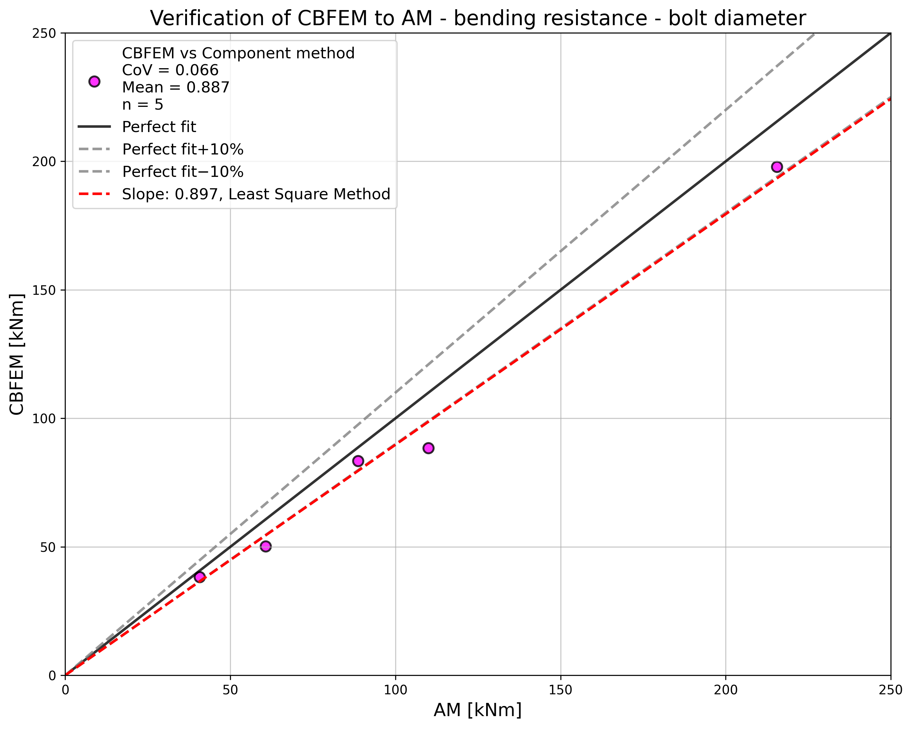
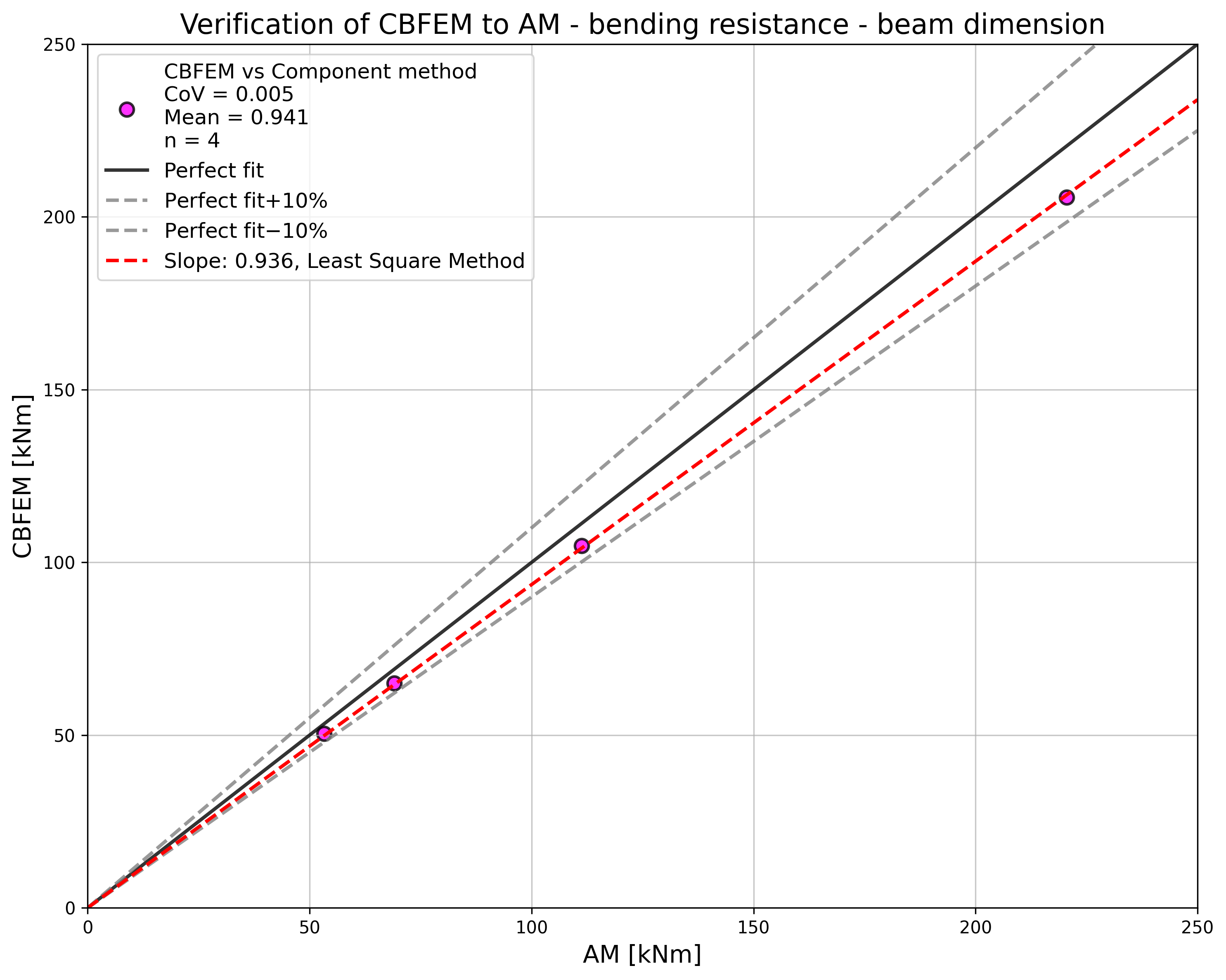
\[ \textsf{\textit{\footnotesize{Fig. 5.5.6 Verification of CBFEM to AM for the interaction of shear and tension in bolt in case of loading to bending resistance of a joint}}}\]

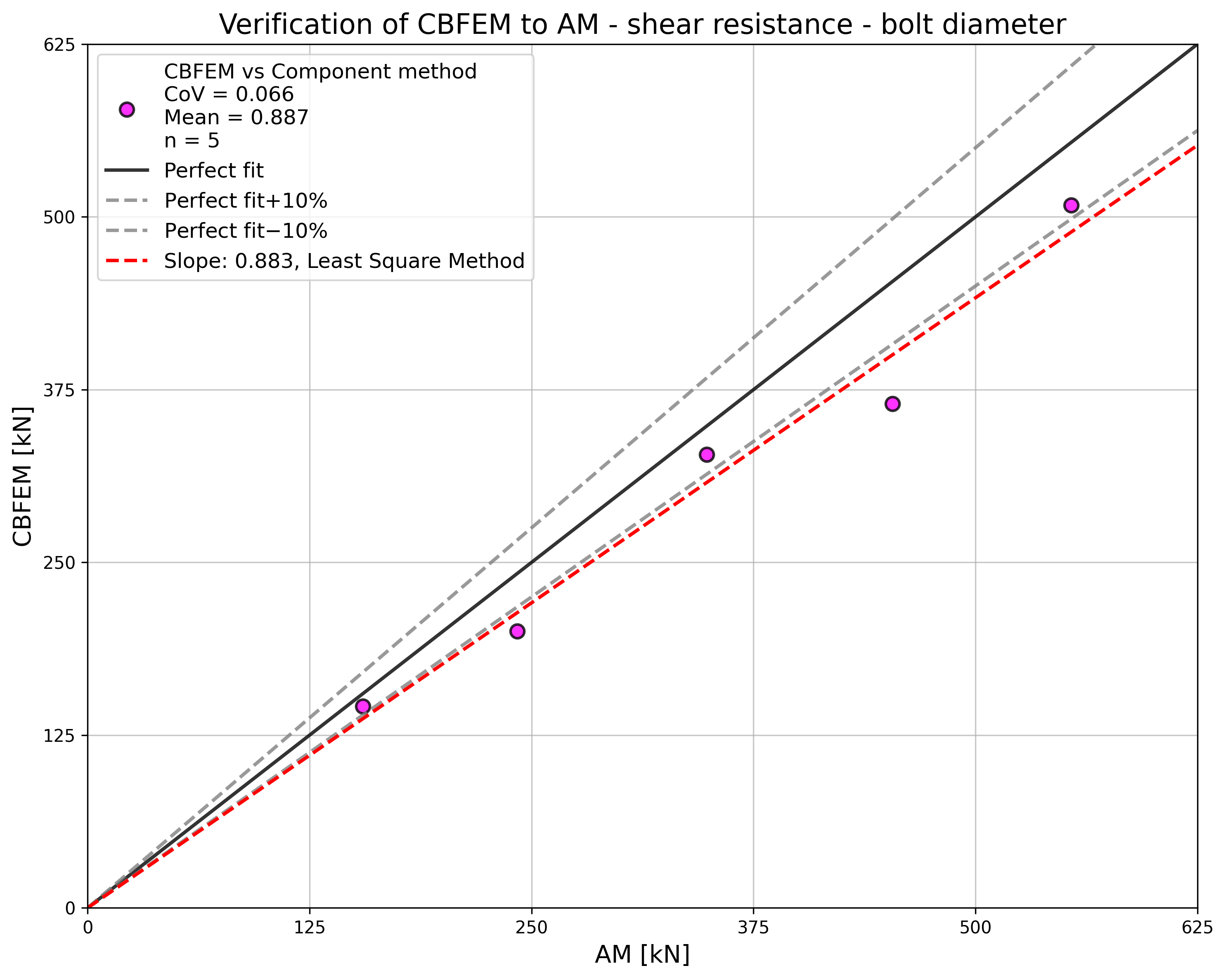
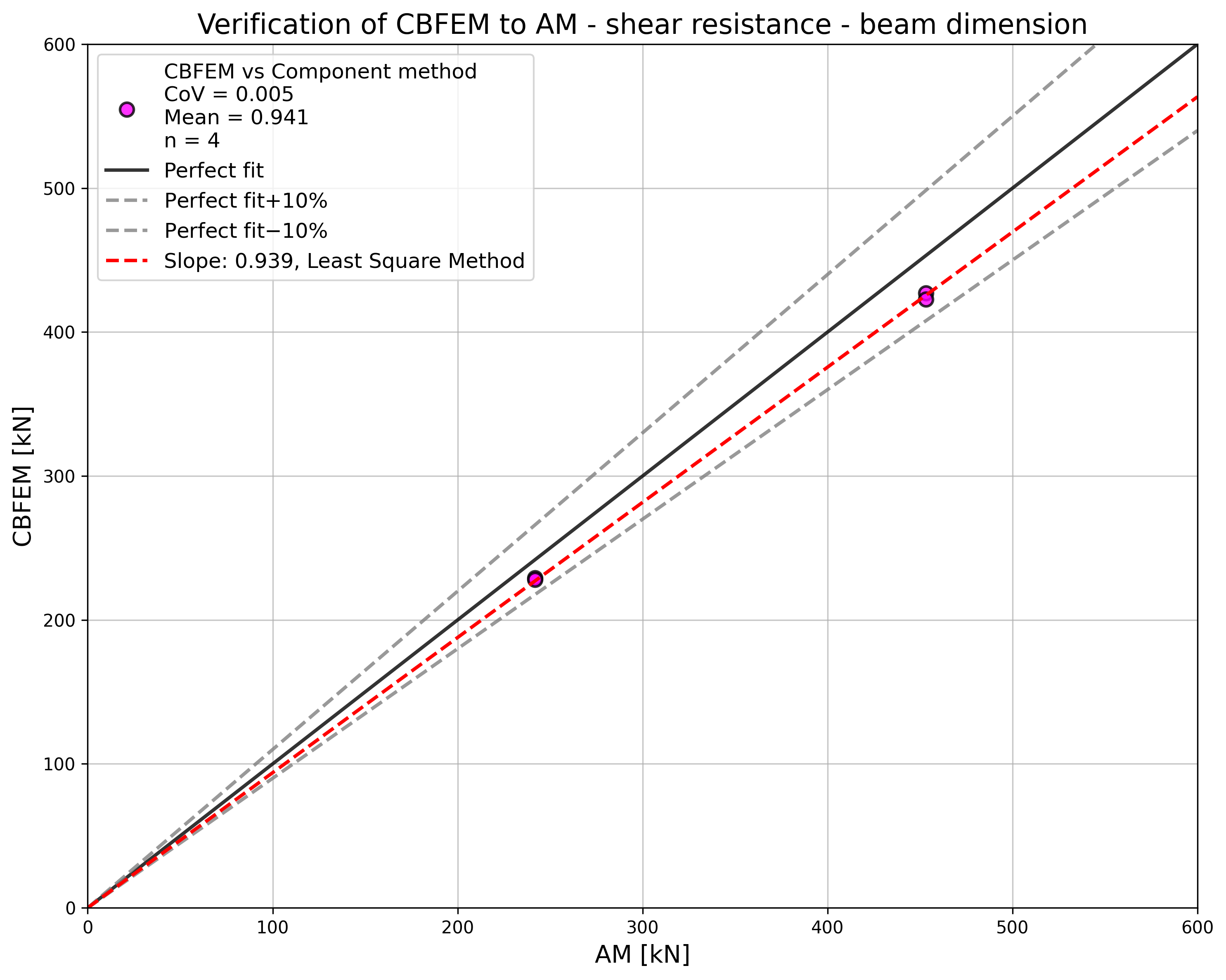
\[ \textsf{\textit{\footnotesize{Fig. 5.5.7 Verification of CBFEM to AM for the interaction of shear and tension in bolt in case of loading to shear resistance of a joint}}}\]

Exemplu de referință

Date de intrare

Elemente conectate

• Oțel S355
• Grinzi HEA300
• Grosimea plăcii de capăt t_p = 40 mm
• Dimensiunile plăcii de capăt 300 × 330 mm

Șuruburi

• 4 × M24 8.8
• Distanțe e₁ = 85 mm; p₁ = 160 mm; w₁ = 75 mm; w = 150 mm

Rezultate

• Rezistența de calcul la încovoiere M_Rd = 93 kNm
• Rezistența de calcul la forfecare V_Rd = 291 kN
• Modul de cedare este cedarea șurubului la interacțiunea dintre forfecare și întindere

Îmbinări la forfecare în îmbinare rezistentă la alunecare

Descriere

Acest studiu este axat pe verificarea metodei elementelor finite bazate pe componente (CBFEM) pentru rezistența îmbinării simetrice duble cu eclise rezistente la alunecare, comparativ cu un model analitic (MA).

Model analitic

Rezistența la alunecare a unui bulон pretensionat este calculată conform capitolului 3.9.1 din EN 1993-1-8:2005. Forța de pretensionare este luată la 70% din rezistența ultimă a bulonului conform ecuației (3.7).

Verificarea rezistenței

Rezistențele de calcul determinate prin CBFEM sunt comparate cu rezultatele modelului analitic (MA); a se vedea (Wald et al. 2018). Rezultatele sunt rezumate în Tab. 5.5.1. Parametrul este diametrul bulonului; a se vedea Fig. 5.5.1.

\[ \textsf{\textit{\footnotesize{Drawing 5.5.1 Joint geometry and dimensions}}}\]

Tab. 5.5.1 Comparație a rezistenței bulonului estimată prin modelul EF față de cea analitică pentru diametrul bulonului; rost: eclisă 200/12 mm, buloane 2 × M× 8.8, plăci 2 × 200/20 mm, oțel S235

Parametru		Model Analitic (MA)	CBFEM		MA/ CBFEM
Diam.	Distanțe	Rezist. [kN]	Componentă critică	Rezist. [kN]	Componentă critică
M16	p = 55 e1 = 40	211	Alunecare	205	Alunecare	1,03
M20	p = 70 e1= 50	329	Alunecare	320	Alunecare	1,03
M24	p = 80 e1 = 60	474	Alunecare	463	Alunecare	1,02
M27	p = 90 e1 = 70	617	Alunecare	596	Alunecare	1,04
M30	p = 100 e1 = 75	754	Alunecare	728	Alunecare	1,04

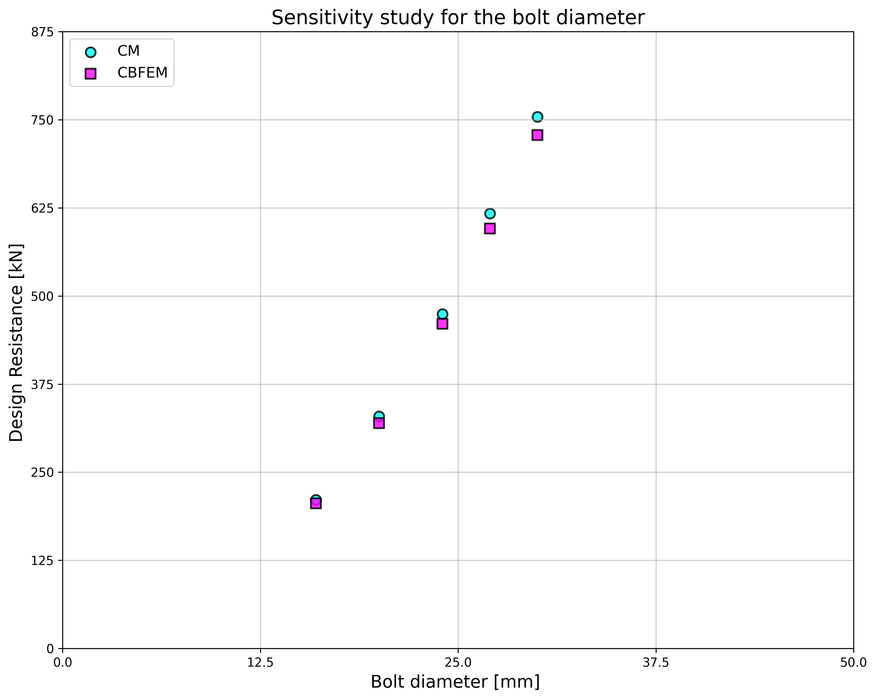
\[ \textsf{\textit{\footnotesize{Fig. 5.5.1 Sensitivity study for the bolt diameter}}}\]

Rezultatele studiilor de sensibilitate sunt rezumate în graficul din Fig. 5.5.2. Rezultatele arată că diferențele dintre cele două metode de calcul sunt sub 5 %. Modelul analitic oferă în general o rezistență mai mare.

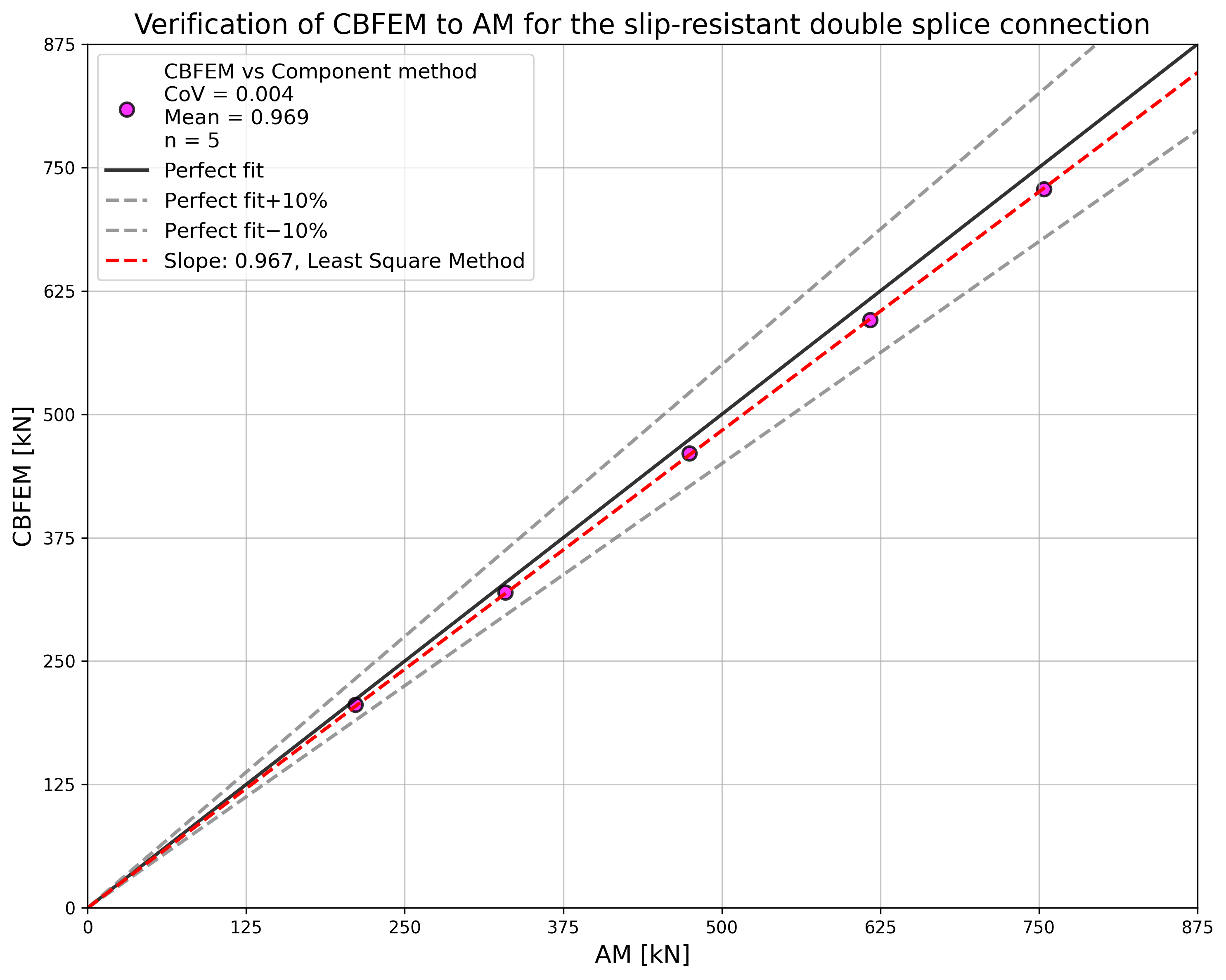
\[ \textsf{\textit{\footnotesize{Fig. 5.5.2 Verification of CBFEM to AM for the slip-resistant double splice connection}}}\]

Exemplu de referință

Date de intrare

Element conectat

• Oțel S235
• Eclisă 200×12 mm

Conectori

Buloane

• 3 × M20 8.8
• Distanțe e₁ = 50 mm, p = 70 mm

Două eclise

• Oțel S235
• Placă 480×200×20 mm

Configurare cod

• Coeficient de frecare la rezistența la alunecare 0,5

Date de ieșire

• Rezistența de calcul F_Rd = 320 kN
• Modul de cedare de calcul este alunecarea buloanelor

\[ \textsf{\textit{\footnotesize{Fig. 5.5.3 Benchmark example of the bolted splices in shear}}}\]

Rezistența la forfecare în bloc

Descriere

Acest capitol este axat pe verificarea metodei elementelor finite bazate pe componente (CBFEM) pentru rezistența la forfecare în bloc a îmbinărilor cu șuruburi solicitate la forfecare, comparativ cu modelul de elemente finite orientat spre cercetare (ROFEM) validat și cu principalele modele analitice (AM).

Model analitic

Există mai multe modele analitice pentru rezistența la forfecare în bloc a îmbinărilor cu șuruburi. Sunt investigate modelele din codurile EN 1993-1-8:2005, EN 1993-1-8:2020, AISC 360-10 și CSA S16-9. De asemenea, în comparație sunt utilizate modelele analitice ale lui Driver et al. (2005) și Topkaya et al. (2004).

\[V_{\mathrm{eff,1,Rd}} = \frac{f_\mathrm{u} A_\mathrm{nt}}{\gamma_\mathrm{M2}} + \left(\frac{1}{\sqrt{3}}\right)\frac{f_\mathrm{y} A_\mathrm{nv}}{\gamma_\mathrm{M0}}\]

\[V_{\mathrm{eff,2,Rd}} = 0.5 \cdot \frac{f_\mathrm{u} A_\mathrm{nt}}{\gamma_\mathrm{M2}} + \left(\frac{1}{\sqrt{3}}\right) \frac{f_\mathrm{y} A_\mathrm{nv}}{\gamma_\mathrm{M0}}\]

\[V_{\mathrm{eff,1,Rd}} =\left[A_\mathrm{nt} f_\mathrm{u} + \min \left(\frac{A_\mathrm{gv} \cdot f_\mathrm{y}}{\sqrt{3}} \; ; \;\frac{A_\mathrm{nv} f_\mathrm{u}}{\sqrt{3}}\right)\right] \bigg/ \gamma_\mathrm{M2}\]

\[V_{\mathrm{eff,2,Rd}} =\left[0.5 A_\mathrm{nt} f_\mathrm{u} + \min \left(\frac{A_\mathrm{gv} \cdot f_\mathrm{y}}{\sqrt{3}}\;;\;\frac{A_\mathrm{nv} f_\mathrm{u}}{\sqrt{3}}\right)\right] \bigg/ \gamma_\mathrm{M2}\]

\[\varphi R_\mathrm{n} =\varphi \left(0.6 f_u A_\mathrm{nv} + U_\mathrm{bs} f_\mathrm{u} A_\mathrm{nt}\right)\leq 0.6 f_\mathrm{y} A_\mathrm{gv} + U_\mathrm{bs} f_\mathrm{u} A_\mathrm{nt}\]

\[T_\mathrm{r} =\varphi_\mathrm{u} \left[U_t A_\mathrm{nt} f_\mathrm{u} + 0.6 A_\mathrm{gv} \frac{f_\mathrm{y} + f_\mathrm{u}}{2} \right]\]

unde:

\(f_\mathrm{y}\) - limita de curgere

\(f_\mathrm{u}\) - rezistența la rupere

\(\gamma_{\mathrm{M2}}\),  \(\varphi_\mathrm{u}\), \(\varphi\) - factori de siguranță

Pentru \(A_\mathrm{nt}\), \(A_\mathrm{nv}\), \(A_\mathrm{gv}\) a se vedea Fig. 5.6.1.

\[ \textsf{\textit{\footnotesize{Fig. 5.6.1 Planele de cedare la forfecarea în bloc}}}\]

Validarea și verificarea rezistenței

Experimentele lui Huns et al. (2002) sunt utilizate pentru validarea ROFEM creat de Sekal (2019) în software-ul ANSYS, a se vedea Fig. 5.6.2. Se utilizează diagrama material tensiune-deformație reală. Sunt modelate doar plăcile cele mai subțiri, destinate să cedeze. Șuruburile sunt simplificate ca deplasări de reazem doar pe semicercul găurii de șurub. Deplasările în toate găurile sunt cuplate. Modelul ROFEM prezintă o concordanță foarte bună cu rezultatele experimentale.

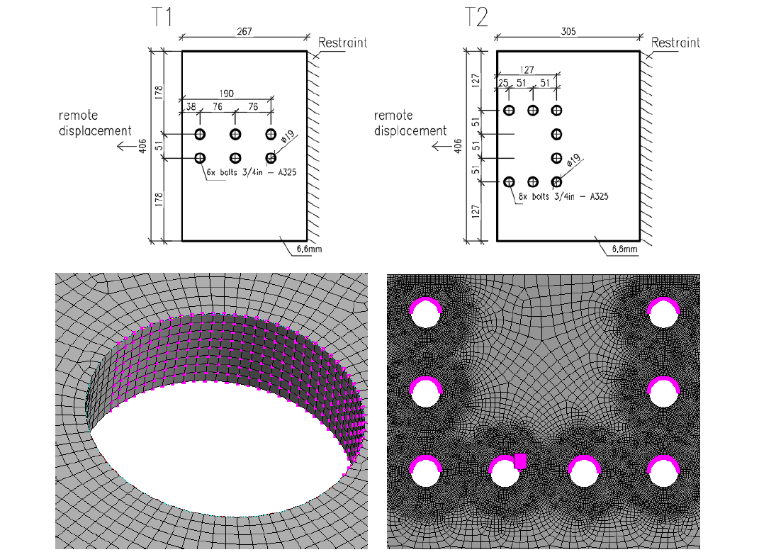
\[ \textsf{\textit{\footnotesize{Fig. 5.6.2 ROFEM cu plasă fină a epruvetelor testate de Huns et al. (Sekal, 2019)}}}\]

Modelul CBFEM orientat spre proiectare utilizează elemente de tip placă cu o plasă relativ grosieră. Plasa este predefinită în apropierea găurilor de șurub. Șuruburile sunt modelate ca arcuri neliniare conectate la nodurile de la marginile găurilor de șurub prin legături. Pentru plăci se utilizează diagrama material biliniară cu ecruisare neglijabilă. Rezistența limită a unui grup de șuruburi la presiune pe gaură este determinată atunci când deformația plastică a plăcii atinge 5% (EN 1993-1-5: 2005). Rezistențele la presiune pe gaură și la sfâșierea găurii pentru fiecare șurub în parte sunt verificate prin formulele din codul corespunzător.

\[ \textsf{\textit{\footnotesize{Fig. 5.6.3 Compararea epruvetei T2 testată de Huns et al. (Sekal, 2019)}}}\]

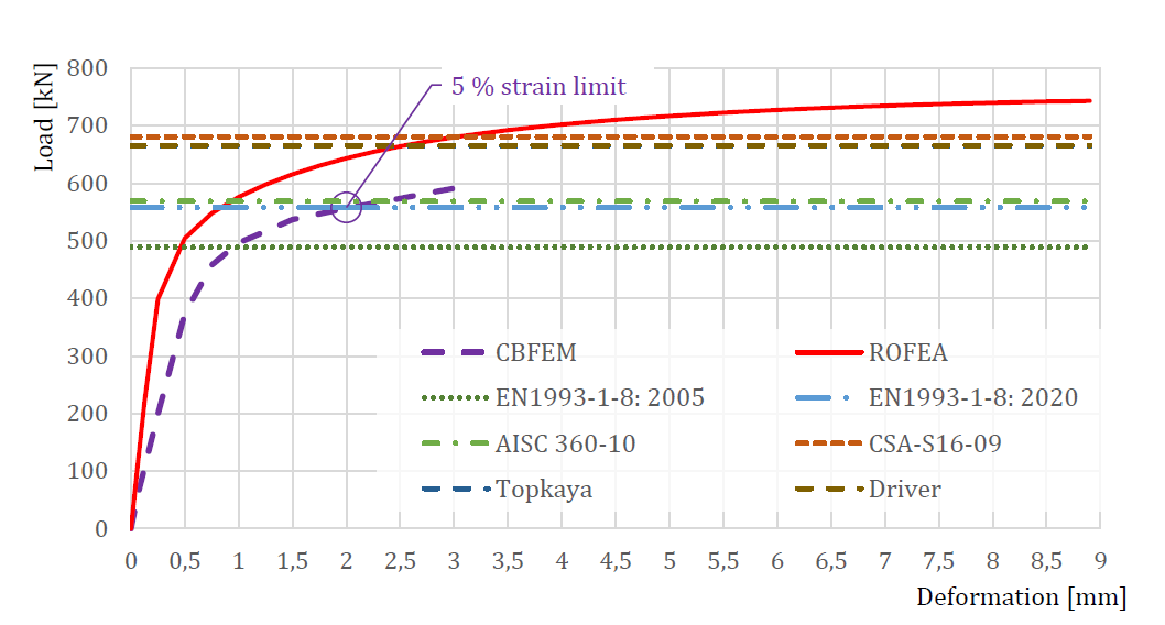
Comparația dintre ROFEM, CBFEM și modelele analitice este prezentată în Fig. 5.6.3. Cel mai conservator este modelul din EN 1993-1-8: 2005, deoarece, spre deosebire de celelalte modele, utilizează planul de forfecare net în combinație cu limita de curgere. Curgerea în planul de forfecare brut este observată în experimente și în modelele numerice. În următoarea generație a prEN 1993-1-8:2022, formula pentru rezistența la forfecare în bloc va fi modificată. Rigiditatea modelului CBFEM este mai mică comparativ cu ROFEM. În experimente, găurile au fost executate cu același diametru ca și șuruburile, astfel încât nu a existat alunecare inițială. Modelul ROFEM ignoră, de asemenea, orice alunecare, însă în CBFEM modelul de forfecare al șuruburilor este aproximat cu ipoteza găurilor standard pentru șuruburi.

Studiu de sensibilitate

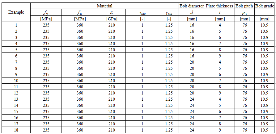
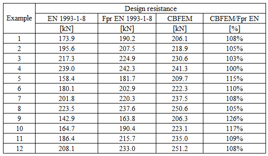
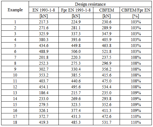
Epruveta T1 a fost utilizată pentru studiul modului în care pasul șuruburilor, Fig. 5.6.4, și grosimea plăcii, Fig. 5.6.6, influențează rezistența la forfecare în bloc. Modelele furnizează rezultate așteptate. Tabelele 5.6.1 și 5.6.2 prezintă o sinteză a exemplelor. Desenul 5.6.1 prezintă geometria și dimensiunile rostului. Rezultatele verificării sunt prezentate în Tabelele 5.6.3 și 5.6.4 și în Fig. 5.6.5., Fig. 5.6.7.

Tabelul 5.6.1 Sinteză exemple. Efectul pasului șuruburilor

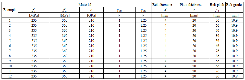
Tabelul 5.6.2 Sinteză exemple. Efectul grosimii plăcii

\[ \textsf{\textit{\footnotesize{Desenul 5.6.1 Geometria și dimensiunile rostului}}}\]

Efectul pasului șuruburilor

Tabelul 5.6.3 Compararea rezultatelor rezistențelor de calcul estimate prin CBFEM, EN 1993-1-8 și Fpr EN 1993-1-8. Efectul pasului șuruburilor

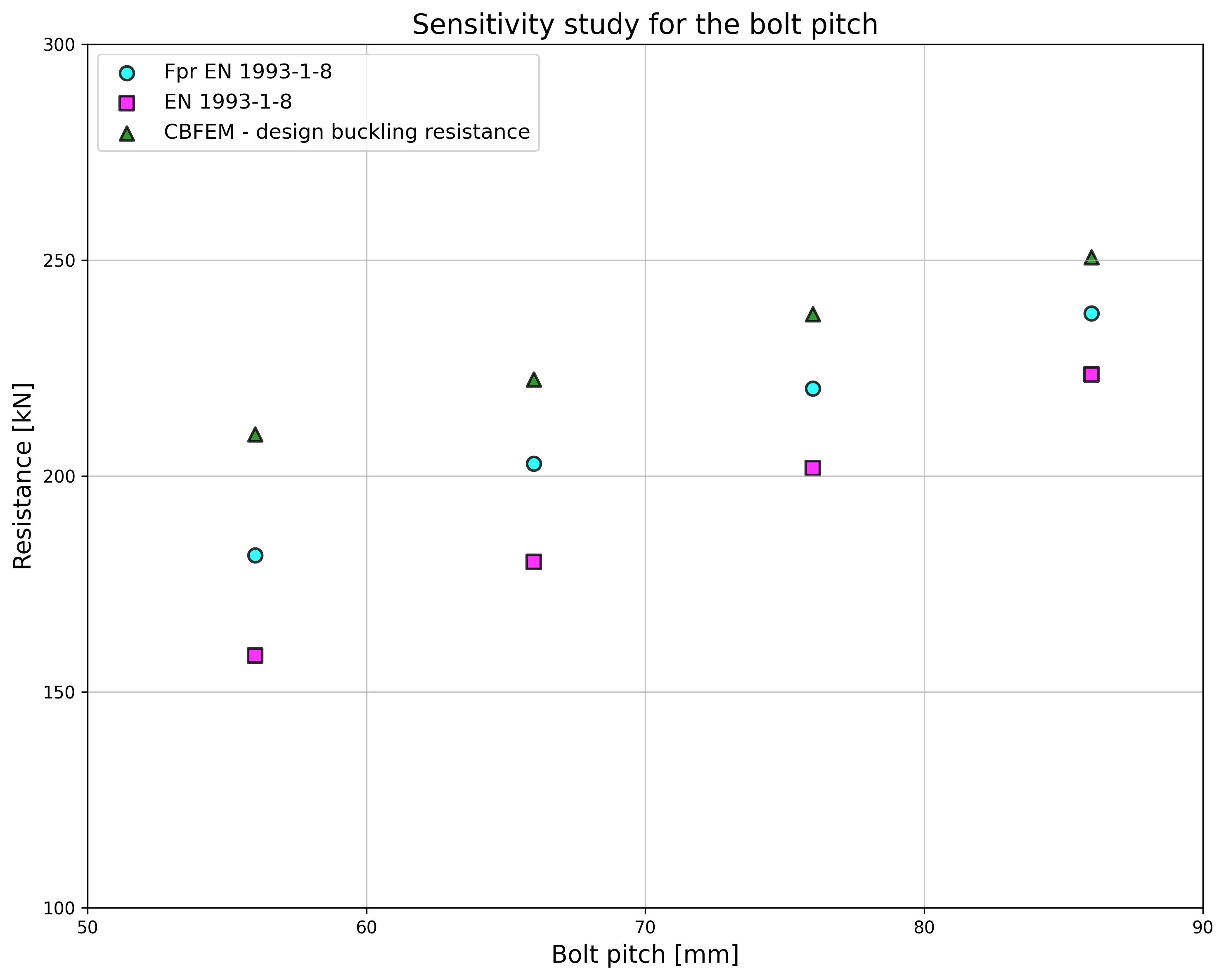
\[ \textsf{\textit{\footnotesize{Fig. 5.6.4 Efectul pasului șuruburilor}}}\]

\[ \textsf{\textit{\footnotesize{Fig. 5.6.5 Verificarea rezistenței determinate prin CBFEM față de Fpr EN 1993-1-8}}}\]

Efectul grosimii plăcii

Tabelul 5.6.4 Compararea rezultatelor rezistențelor de calcul estimate prin CBFEM, EN 1993-1-8 și Fpr EN 1993-1-8. Efectul grosimii plăcii

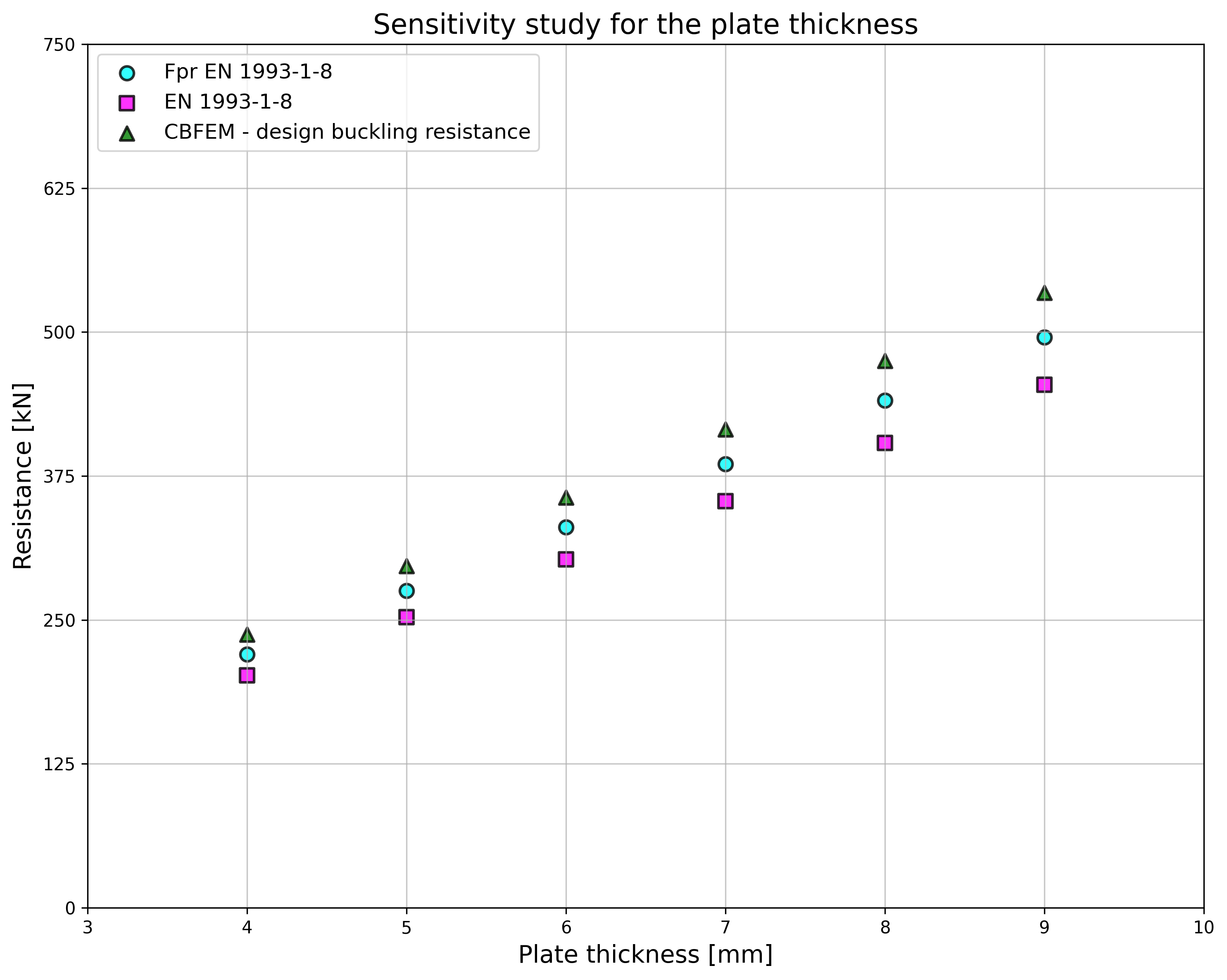
\[ \textsf{\textit{\footnotesize{Fig. 5.6.6 Efectul grosimii plăcii}}}\]

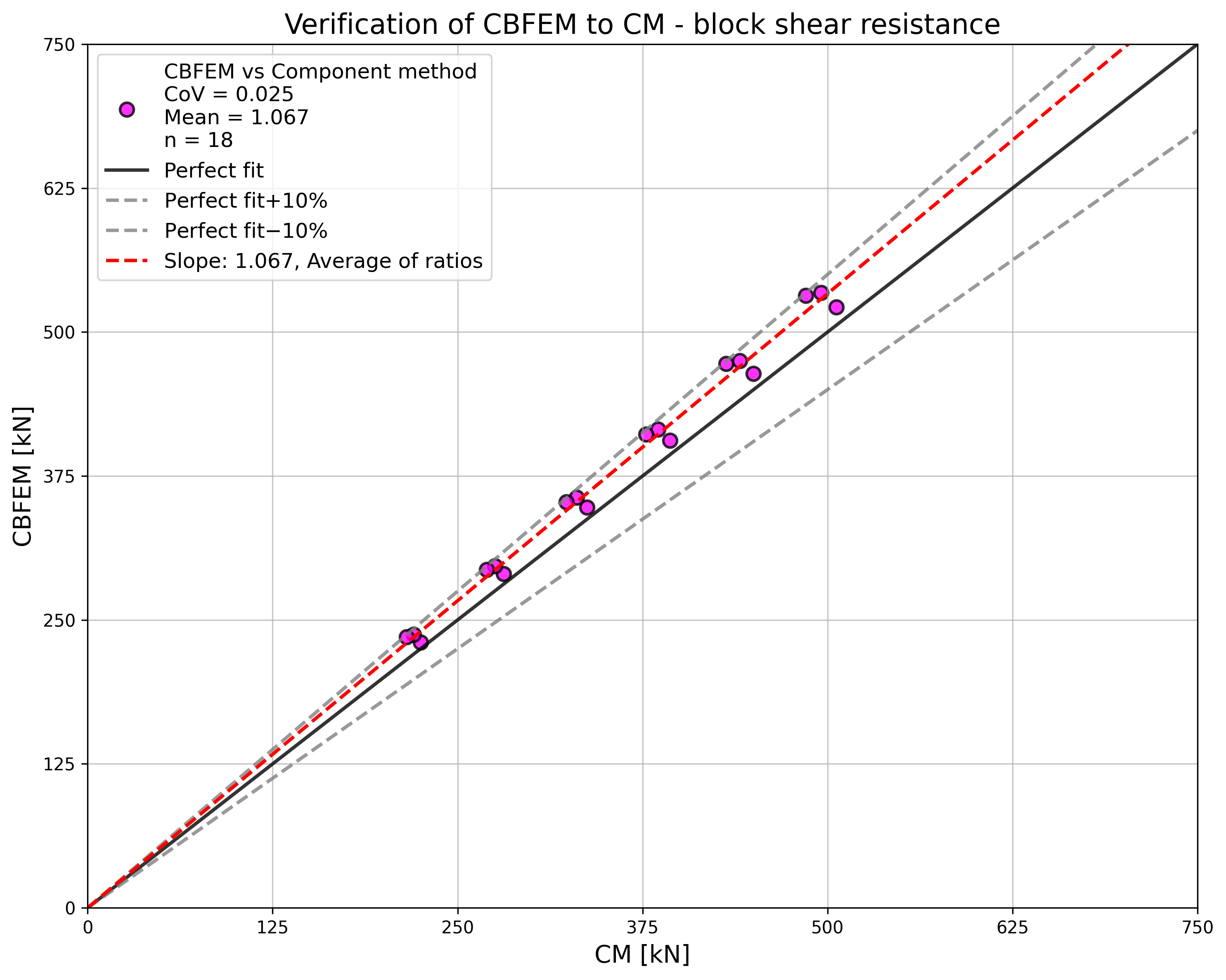
\[ \textsf{\textit{\footnotesize{Fig. 5.6.7 Verificarea rezistenței determinate prin CBFEM față de Fpr EN 1993-1-8}}}\]

Exemplu de referință

Date de intrare

 Element

• Oțel S450
• Profil I laminat
• b = 300mm
• h = 19mm
• t_f = 7mm
• t_w = 6.2mm

Placă - element de reazem

• Oțel S235
• b = 400mm
• t = 4mm

Șuruburi

• 6 × M16 10.9
• Distanțe e₁ = 38 mm; p₁ = 70 mm; p₂ = 56 mm

Rezultate

• Rezistența de calcul N_Rd = 206.1 kN
• Critică este deformația plastică a plăcii de nod

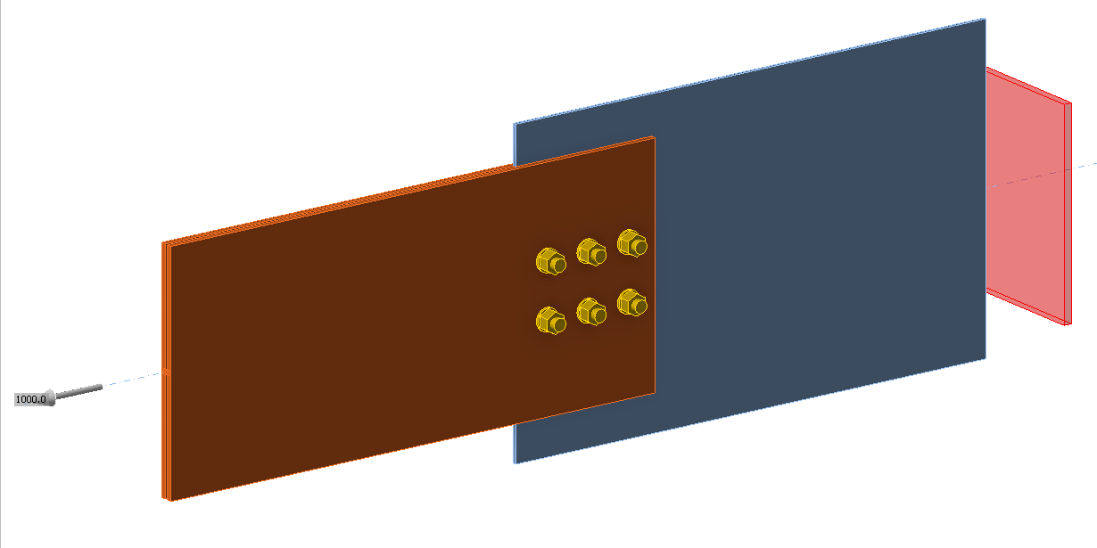
\[ \textsf{\textit{\footnotesize{Fig. 5.6.9 Exemplu de referință}}}\]

Îmbinare cu placă de capăt cu patru șuruburi pe rând

Descriere

Acest studiu este axat pe verificarea metodei elementelor finite bazate pe componente (CBFEM) pentru rezistența îmbinării cu placă de capăt cu patru șuruburi pe rând față de un model analitic (AM) și un model cu elemente finite orientat spre cercetare (ROFEM), validat pe experimente.

Model analitic

Rezistența șuruburilor la forfecare și întindere și rezistența plăcii la presiune pe gaură și la poansonare sunt proiectate conform Tab. 3.4, Capitolul 3.6.1 din EN 1993-1-8:2006. T-stubul echivalent la întindere, conform Capitolului 6.2.4, a fost modificat de Jaspart et al. (2010), a se vedea Fig. 5.7.1 și Tab. 5.7.1.

\[ \textsf{\textit{\footnotesize{Fig. 5.7.1 Moduri de cedare ale T-stubului cu patru șuruburi pe rând: modul 1 (stânga), modul 2 (mijloc), modul 3 (dreapta)}}}\]

Tab. 5.7.1 Moduri de cedare ale T-stubului cu patru șuruburi pe rând (Jaspart et al. 2010)

În Tab. 5.7.1, 𝐹_t,Rd este rezistența de calcul a șurubului la întindere, 𝑒_w=𝑑_w/4, 𝑑_w este diametrul șaibei sau lățimea peste colțuri a capului șurubului sau a piuliței, după caz, 𝑚, 𝑛=𝑒₁+𝑒₂;⁡𝑛≤1.25𝑚, 𝑛₁=𝑒₁, 𝑛₂=𝑒₂;⁡𝑛₂≤1,25𝑚+𝑛₁ a se vedea Fig. 5.8.2, 𝑀_pl,1,Rd=0.25𝑙_eff,1𝑡_f²𝑓_y/𝛾_M0, 𝑀_pl,2,Rd=0.25𝑙_eff,2𝑡_f²𝑓_y/𝛾_M0, 𝑙_eff este lungimea efectivă, 𝑡_f este grosimea tălpii, iar 𝑓_y este limita de curgere, a se vedea Fig. 5.7.2.

\[ \textsf{\textit{\footnotesize{Fig. 5.7.2 Geometria T-stubului cu patru șuruburi pe rând}}}\]

Validarea și verificarea rezistenței

Rezistențele de calcul determinate prin CBFEM au fost comparate cu rezultatele modelului analitic (Zakouřil, 2019) și cu experimentele utilizând modelul cu elemente finite orientat spre cercetare (Samaan et al. 2017), a se vedea Fig. 5.7.3. Rezultatele sunt rezumate în Fig. 5.7.4. S-au utilizat șuruburi de clasa 8.8 și oțel S450. Limitele de curgere și rezistențele la rupere corespund îndeaproape valorilor experimentale, de ex. limita de curgere a șurubului este 600 MPa, rezistența la rupere a șurubului este 800 MPa.

\[ \textsf{\textit{\footnotesize{Placă de capăt extinsă nerigidizată, notată ENS}}}\]

\[ \textsf{\textit{\footnotesize{Placă de capăt înecată, notată F}}}\]

\[ \textsf{\textit{\footnotesize{Placă de capăt extinsă rigidizată, notată EX}}}\]

\[ \textsf{\textit{\footnotesize{Fig. 5.7.3 Epruvete testate}}}\]

Rezistența la moment încovoietor determinată prin CBFEM se situează de obicei între rezistențele determinate prin metoda componentelor și cele obținute experimental. Tabelul 5.7.2 prezintă comparația dintre rezistențele obținute prin CM, CBFEM, ROFEM și experiment pentru epruvetele cu grosimi ale plăcii de capăt de 20 mm și 32 mm. Atât metoda componentelor, cât și CBFEM subestimează rezistența epruvetei cu placă de capăt înecată. 

Tab. 5.7.2 Comparație între CM, ROFEM, CBFEM și experiment

Tabelul 5.7.3 și Fig. 5.7.4 prezintă verificarea CBFEM față de CM pentru modelele ENS cu diferite grosimi ale plăcii de capăt, diametre ale șuruburilor și înălțimi ale grinzii

Tab. 5.7.3 Verificare CBFEM față de CM ENS

\[ \textsf{\textit{\footnotesize{Fig. 5.7.4 Verificarea CBFEM față de CM}}}\]

Rezultatele studiilor de sensibilitate sunt rezumate în graficele din Fig. 5.7.5, Fig. 5.7.6, Fig. 5.7.7 

\[ \textsf{\textit{\footnotesize{Fig. 5.7.5 Studiu de sensibilitate pentru grosimea plăcii}}}\]

\[ \textsf{\textit{\footnotesize{Fig. 5.7.6 Studiu de sensibilitate pentru diametrul șurubului}}}\]

\[ \textsf{\textit{\footnotesize{Fig. 5.7.7 Studiu de sensibilitate pentru înălțimea grinzii}}}\]

Tabelul 5.7.4 și Fig. 5.7.8 prezintă verificarea CBFEM față de CM pentru modelele F cu diferite grosimi ale plăcii de capăt și diametre ale șuruburilor 

Tab. 5.7.4 Verificare CBFEM față de CM F

\[ \textsf{\textit{\footnotesize{Fig. 5.7.8 Verificarea CBFEM față de CM}}}\]

Rezultatele studiilor de sensibilitate sunt rezumate în graficele din Fig. 5.7.9 și 5.7.10

\[ \textsf{\textit{\footnotesize{Fig. 5.7.9 Studiu de sensibilitate pentru grosimea plăcii}}}\]

\[ \textsf{\textit{\footnotesize{Fig. 5.7.10 Studiu de sensibilitate pentru diametrul șurubului}}}\]

Tabelul 5.7.5 și Fig. 5.7.11 prezintă verificarea CBFEM față de CM pentru modelele F cu diferite grosimi ale plăcii de capăt și diametre ale șuruburilor 

Tab. 5.7.5 Verificare CBFEM față de CM EX

\[ \textsf{\textit{\footnotesize{Fig. 5.7.11 Verificarea CBFEM față de CM}}}\]

Rezultatele studiilor de sensibilitate sunt rezumate în graficele din Fig. 5.7.12 și 5.7.13. 

\[ \textsf{\textit{\footnotesize{Fig. 5.7.12 Studiu de sensibilitate pentru grosimea plăcii}}}\]

\[ \textsf{\textit{\footnotesize{Fig. 5.7.13 Studiu de sensibilitate pentru diametrul șurubului}}}\]

Exemplu de referință

Date de intrare

• Oțel S450

Stâlp

• Profil I laminat
• h = 390mm
• b = 350mm
• t_f = 20mm
• t_w = 12mm
• r = 27mm

Rigidizatori stâlp

• t_s = 16mm

Grindă

• Profil I laminat
• h_b = 340mm
• b_b = 350mm
• t_f = 20mm
• t_w = 12mm
• r = 27mm

Placă de capăt

• t_p = 20mm
• b_p = 350mm
• h_p= 540mm

Șuruburi

• 4 rânduri x 4 x M16 8.8
• Distanțe e₁ = 50 mm, p₁ = 120 mm, p₂ = 100mm, e₂= 50mm, w₁ = 75mm, w₂ = 100mm

Suduri

• a_w = 7mm

Rezultate

• Rezistența de calcul F_Rd = 247 kN
• Componentele critice sunt șuruburile cu forțe majorate datorită efectului de pârghie al plăcii de capăt

\[ \textsf{\textit{\footnotesize{Fig. 5.7.14 Exemplu de referință}}}\]

Placă zveltă la compresiune

Vută triunghiulară

Descriere

Obiectul acestui studiu este verificarea metodei elementelor finite bazate pe componente (CBFEM) pentru o vută triunghiulară de clasa 4 fără talpă și o vută triunghiulară de clasa 4 cu talpă cu rigiditate redusă, cu modelul FEM de cercetare (RFEM) și modelul FEM de proiectare (DFEM).

Investigație experimentală

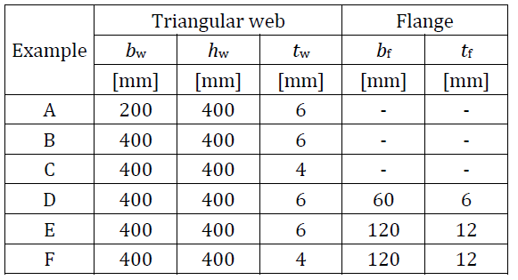
Sunt prezentate rezultatele experimentale ale șase epruvete de vute cu și fără tălpi. Trei epruvete sunt fără tălpi și trei epruvete sunt susținute de tălpi suplimentare. Epruvetele nerigidizate diferă prin grosimea inimii tw și lățimea inimii bw. Epruvetele rigidizate diferă prin grosimea inimii tw, grosimea tălpii tf și lățimea tălpii bf. Dimensiunile epruvetelor sunt rezumate în Tab. 6.1.1. Configurația de testare pentru epruveta fără talpă este prezentată în Fig. 6.1.1 (sus), iar pentru epruveta cu talpă în Fig. 6.1.1 (jos). Caracteristicile materialului plăcilor de oțel sunt rezumate în Tab. 6.1.2.

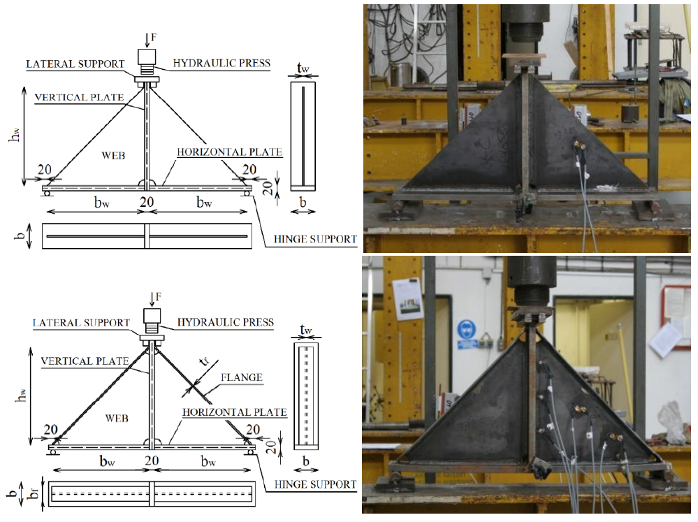
\[ \textsf{\textit{\footnotesize{Fig. 6.1.1 Geometria epruvetelor și configurația de testare}}}\]

Tab. 6.1.1 Prezentare generală a exemplelor

Tab. 6.1.2 Caracteristicile materialelor utilizate în modelele numerice

Modelul FEM de cercetare

Modelul FEM de cercetare (RFEM) este utilizat pentru verificarea modelului DFEM și este validat pe baza experimentelor. În modelul numeric, se aplică elemente de coajă cvadrilaterale cu 4 noduri situate la colțuri, cu o lungime maximă a laturii de 10 mm. Se aplică analiza neliniară material și geometric cu imperfecțiuni (GMNIA). Imperfecțiunile geometrice echivalente sunt derivate din primul mod de flambaj, iar amplitudinea este stabilită conform Anexei C din EN 1993-1-5:2006. Modelele numerice sunt prezentate în Fig. 6.1.2.

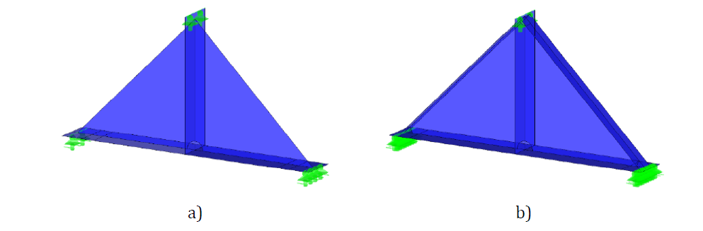
\[ \textsf{\textit{\footnotesize{Fig. 6.1.2 Modelul FEM de cercetare a) vută fără talpă b) vută cu talpă}}\]

Un exemplu de comparație între RFEM și testul experimental privind comportamentul forță-deplasare este prezentat în Fig. 6.1.3a. Comparația rezistențelor măsurate în experiment și obținute din RFEM este prezentată în Fig. 6.1.3b. Rezistența calculată în modelul numeric este afișată pe axa orizontală. Rezistența măsurată în studiul experimental este afișată pe axa verticală. Se poate observa că există o bună concordanță.

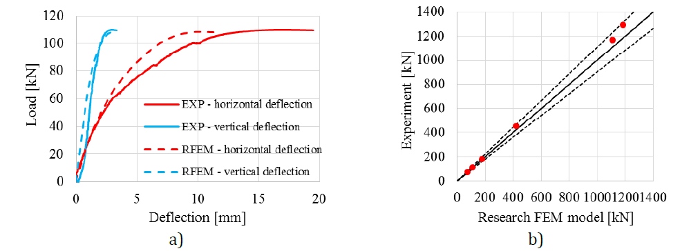
\[ \textsf{\textit{\footnotesize{Fig. 6.1.3 a) Curba forță-deplasare a unei vute fără talpă b) Rezistențele experimentale comparate cu cele din RFEM}}}\]

Comparațiile stărilor finale de deformare între simulările numerice și rezultatele experimentale sunt efectuate la sfârșitul testelor. Fig. 6.1.4 prezintă comparația deformației epruvetelor A, B și D după cedare cu RFEA. Se poate constata că există o bună concordanță între modelele numerice și rezultatele experimentale ale vutelor în ceea ce privește modul de cedare. Pentru mai multe detalii, a se vedea (Kurejková și Wald, 2017).

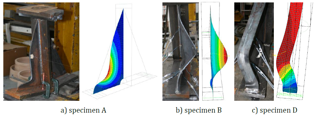
\[ \textsf{\textit{\footnotesize{Fig. 6.1.4 Deflecția experimentală și numerică a epruvetelor A, B și D după cedare}}}\]

Modelul FEM de proiectare

Procedura de proiectare pentru secțiunile transversale de clasa 4 este descrisă în secțiunea 3.10 Flambaj local.
Procedura de proiectare este verificată prin compararea modelelor DFEM și RFEM. Ambele modele sunt create în software-ul Dlubal RFEM. Procedura este aplicată în modelele CBFEM; a se vedea (Kurejková et al. 2015). Rezistența determinată de 5% deformație plastică este obținută în primul pas, urmată de analiza liniară de flambaj. Componenta critică în analiza de flambaj este studiată. Rezistența de calcul este interpolată până când condiția ρ∙α_ult,k = 1 este îndeplinită.

Primul mod de flambaj al unei vute fără talpă este prezentat în Fig. 6.1.5 a). Rezistența este evaluată conform formulei (3.10.2) din secțiunea 3.10. Comparația rezistențelor DFEM și RFEM este prezentată în Fig. 6.1.5 b). Rezistența calculată în DFEM este afișată pe axa orizontală. Rezistența calculată în RFEM este afișată pe axa verticală. Se poate observa că există o bună concordanță și că procedura este verificată.

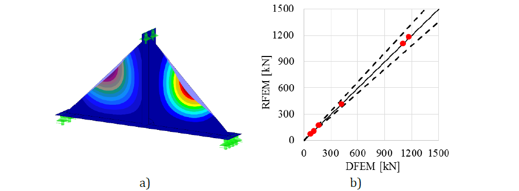
\[\textsf{\textit{\footnotesize{Fig. 6.1.5 a) Primul mod de flambaj al modelului DFEM b) Comparația rezistențelor DFEM și RFEM}}}\]

Comportament global și verificare

Este pregătită o comparație a comportamentului global al unei vute fără talpă descris prin diagrame forță-deplasare în modelul DFEM. Deplasarea este măsurată în direcție verticală în mijlocul epruvetei. Atenția este concentrată pe caracteristicile principale: rezistența de calcul și sarcina critică. Două exemple de vute fără talpă sunt alese ca referință; a se vedea Fig. 6.1.6. Procedura de proiectare în modelele DFEM acoperă rezerva post-flambaj, care este observată în Fig. 6.1.6 a). Sarcina critică Fcr este mai mică decât rezistența de calcul FDFEM. Rezerva post-flambaj este observată în cazurile cu plăci foarte zvelte. Diagrama tipică este prezentată în Fig. 6.1.6 b), unde rezistența de calcul FDFEM nu atinge sarcina critică Fcr. Sarcina Fult,k se referă la rezistența corespunzătoare unui procent de 5% deformație plastică.

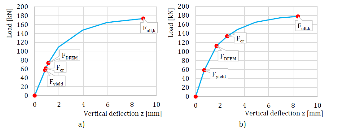
\[ \textsf{\textit{\footnotesize{Fig. 6.1.6 a) Curba forță-deplasare cu rezervă post-flambaj b) Curba forță-deplasare fără rezervă post-flambaj (Kuříková et al. 2019)}}}\]

Procedura de proiectare în modelele CBFEM este descrisă în secțiunea 3.10 Flambaj local. Analiza de flambaj este implementată în software. Calculul rezistențelor de calcul se efectuează manual conform procedurii de proiectare. FCBFEM este interpolat de utilizator până când formula (2) este egală cu 1. Este studiat un nod grindă-stâlp cu o vută fără talpă. Grosimile inimilor grinzii și stâlpului variază în același mod ca și grosimea vutei triunghiulare. Aceeași secțiune transversală este utilizată pentru grindă și stâlp. Geometria exemplelor este descrisă în Tab. 6.1.3. Nodul este încărcat cu moment încovoietor.

Tab. 6.1.3 Prezentare generală a exemplelor (Kuříková et al. 2019)

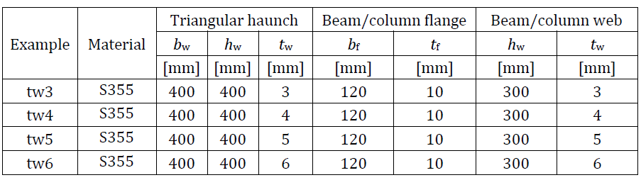
Verificarea rezistenței

Rezistența de calcul calculată prin CBFEM este comparată cu rezultatele obținute prin RFEM. Comparația este axată pe rezistența de calcul și sarcina critică. Rezultatele sunt prezentate în Tab. 6.1.4. Diagrama din Fig. 6.1.7 c) prezintă influența grosimii elementului de lărgire asupra rezistențelor și sarcinilor critice în exemplele examinate.
Rezultatele arată o concordanță foarte bună în ceea ce privește sarcina critică și rezistența de calcul. Rezerva post-flambaj este observată pentru inima grinzii și elementul de lărgire triunghiular cu grosimi de 3 și 4 mm. Modelul CBFEM al nodului cu o vută cu grosimea de 3 mm este prezentat în Fig. 6.1.7 a). Primul mod de flambaj al nodului este prezentat în Fig. 6.1.7 b).

Tab. 6.1.4 Rezistența de calcul

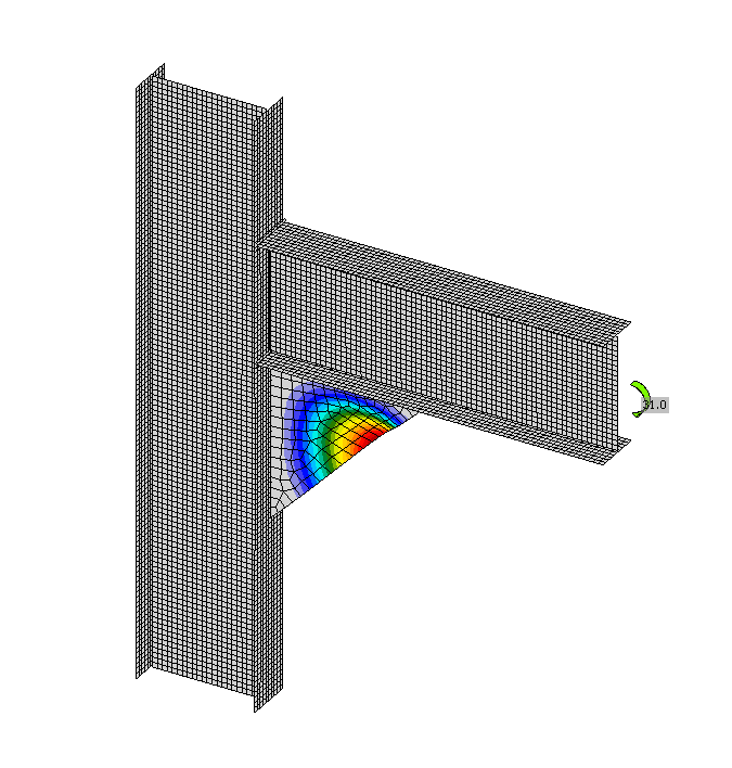
\[ \textsf{\textit{\footnotesize{a)}}}\]

\[ \textsf{\textit{\footnotesize{b)}}}\]

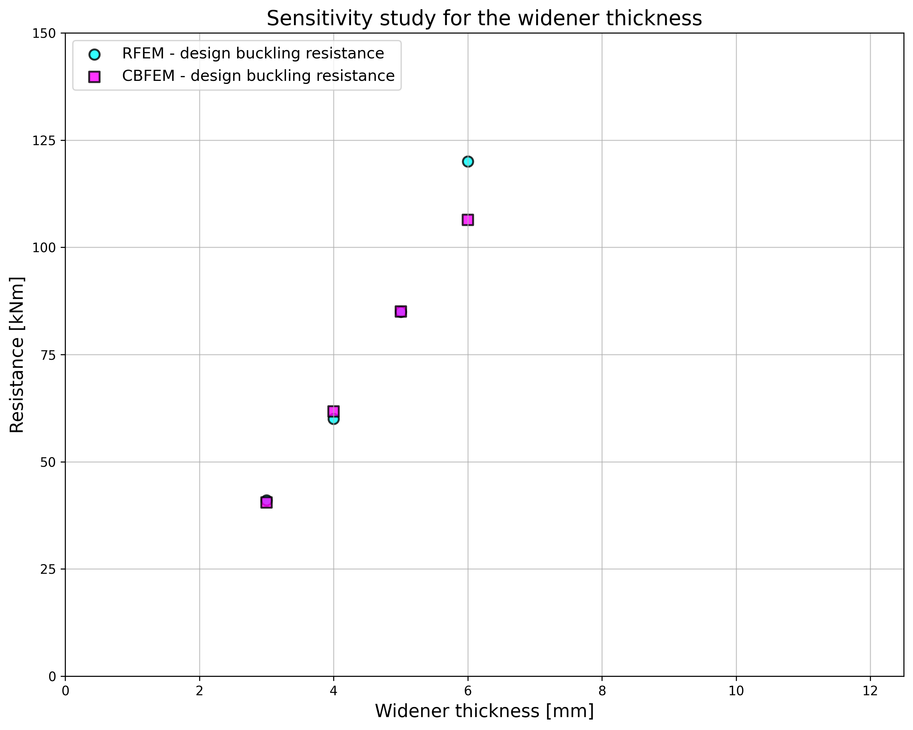
\[ \textsf{\textit{\footnotesize{c)}}}\]

\[ \textsf{\textit{\footnotesize{Fig. 6.1.7 a) Primul mod de flambaj b) Modelul CBFEM c) Influența grosimii elementului de lărgire asupra rezistențelor și sarcinilor critice}}}\]

Studiile de verificare confirmă acuratețea modelului CBFEM pentru predicția comportamentului unei vute triunghiulare. Rezultatele CBFEM sunt comparate cu rezultatele RFEM. Procedura de proiectare este verificată pe modelul RFEM, care este validat pe experimente. Toate procedurile prezic un comportament global similar al nodului.

Exemplu de referință

Date de intrare

Grindă și stâlp
• Oțel S355
• Grosimea tălpii tf = 10 mm
• Lățimea tălpii bf = 120 mm
• Grosimea inimii tw = 3 mm
• Înălțimea inimii hw = 300 mm

Vută triunghiulară
• Grosimea tw = 3 mm
• Lățimea bw = 400 mm
• Înălțimea hw = 400 mm

Calculați
• Analiza de flambaj

Date de ieșire

 • Rezistența plastică CBFEM = 138 kNm
•   Rezistența de calcul la flambaj CBFEM = 41 kNm
• Factorul critic de flambaj (pentru Rezistența de calcul la flambaj CBFEM = 41 kNm) αcr = 0,52
• Factorul de încărcare la 5% deformație plastică α_ult,k = Rezistența plastică CBFEM / Rezistența de calcul la flambaj CBFEM = 138 / 41 = 3,40

\[ \textsf{\textit{\footnotesize{Fig. 6.1.7 Vută triunghiulară calculată în exemplul de referință}}}\]

Panoul inimii stâlpului la forfecare

Descriere

Obiectivul acestui studiu este verificarea metodei elementelor finite bazate pe componente (CBFEM) a unei îmbinări grindă-stâlp cu o inimă de stâlp de clasa 4 prin metoda componentelor (CM).

Model analitic

Componenta panou al inimii stâlpului la forfecare este descrisă în cl. 6.2.6.1 din EN 1993-1-8:2005. Metoda de calcul este limitată la zveltețea inimii stâlpului d / t_w ≤ 69 ε. Inimile cu zveltețe mai mare se calculează conform EN 1993-1-5:2006 cl. 5 și Anexa A. Rezistența la forfecare este compusă din rezistența la flambaj prin forfecare a panoului inimii și rezistența cadrului format din tălpi și elementele de rigidizare care înconjoară panoul. Rezistența la flambaj a panoului inimii se bazează pe tensiunea critică de forfecare

\[ \tau_{cr} = k_{\tau} \sigma_E \]

unde σ_E este tensiunea critică Euler a plăcii

\[ \sigma_E = \frac{\pi^2 E}{12 (1-\nu^2)} \left ( \frac{t_w}{h_w} \right )^2 \]

Coeficientul de flambaj k_τ se obține din EN 1993-1-5:2006, Anexa A.3.

Zveltețea panoului inimii este

\[ \bar{\lambda_w} = 0.76 \sqrt{\frac{f_{yw}}{\tau_{cr}}} \]

Factorul de reducere χ_w se poate obține din EN 1993-1-5:2006 cl. 5.3.

Rezistența la flambaj prin forfecare a panoului inimii este

\[ V_{bw,Rd} = \frac{\chi_w f_{yw} h_w t_w}{\sqrt{3} \gamma_{M1}} \]

Rezistența cadrului poate fi calculată conform cl. 6.2.6.1 din EN 1993-1-8:2005.

Modelul de calcul cu elemente finite

Procedura de calcul pentru plăci zvelte este descrisă în secțiunea 3.10. Analiza liniară de flambaj este implementată în software. Calculul rezistențelor de calcul se efectuează conform procedurii de calcul. F_CBFEM este interpolat de utilizator până când ρ ∙ α_ult,k/γ_M1 este egal cu 1.

Se studiază o îmbinare grindă-stâlp cu o inimă de stâlp zveltă. Înălțimea inimii grinzii variază; astfel, lățimea panoului inimii stâlpului variază. Geometria exemplelor este descrisă în Tab. 6.2.1. Îmbinarea este încărcată cu moment încovoietor.

Tab. 6.2.1 Prezentare generală a exemplelor

Exemplu	Talpă stâlp		Inimă stâlp		Grindă	Material
	bf	tf	hw	tw	IPE
	[mm]	[mm]	[mm]	[mm]
IPE400	250	10	820	4	400	S235
IPE 450	250	10	820	4	450	S235
IPE500	250	10	820	4	500	S235
IPE 550	250	10	820	4	550	S235
IPE600	250	10	820	4	600	S235

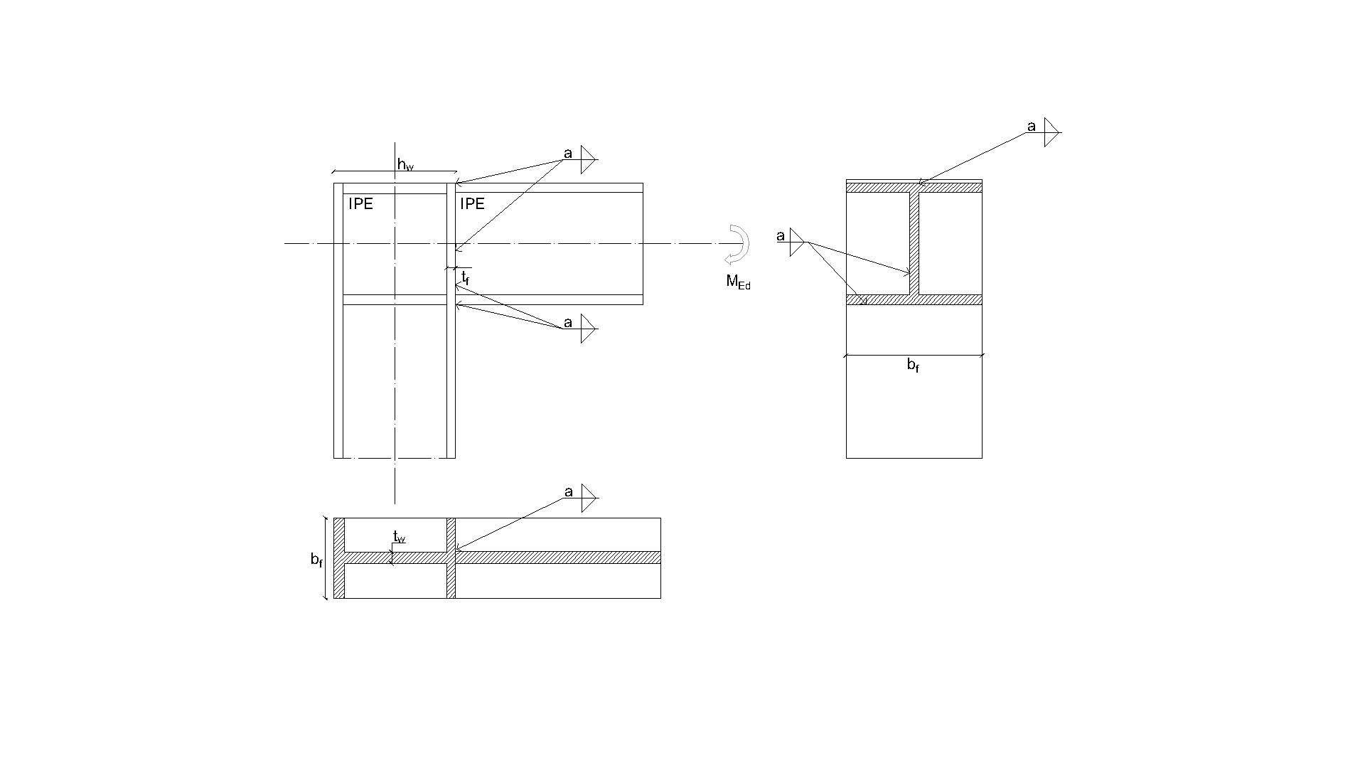
\[ \textsf{\textit{\footnotesize{Fig. 6.2.1 Geometria și dimensiunile îmbinării}}}\]

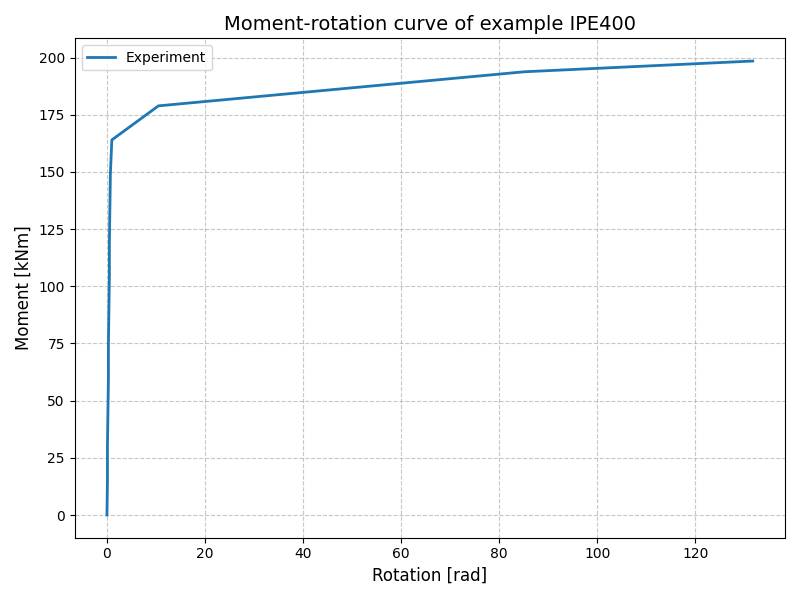
\[ \textsf{\textit{\footnotesize{Fig. 6.2.2 Curba moment-rotație pentru exemplul IPE400}}}\]

Comportament global și verificare

Comportamentul global al unei îmbinări grindă-stâlp cu o inimă de stâlp zveltă, descris prin diagrama moment-rotație în modelul CBFEM, este prezentat în Fig. 6.2.2. Atenția este concentrată pe caracteristicile principale: rezistența de calcul și sarcina critică. Diagrama este completată cu un punct în care începe curgerea și rezistența la 5 % deformație plastică.

Verificarea rezistenței

Rezistența de calcul calculată prin CBFEM este comparată cu CM. Comparația este axată pe rezistența plastică. Rezultatele sunt prezentate în Tab. 6.2.2a. Fig. 6.2.2a prezintă diferențele dintre cele două metode de calcul. Tabelul 6.2.2b prezintă datele privind rezistența de calcul la flambaj. Tabelul 6.2.2c și Fig. 6.2.3c prezintă diferențele dintre cele două metode de calcul la determinarea rezistenței la flambaj. Diagrama din Fig. 6.2.3c prezintă influența înălțimii secțiunii grinzii asupra rezistențelor și sarcinilor critice în exemplele analizate.

Tab. 6.2.2a Rezistențe plastice ale CM și CBFEM

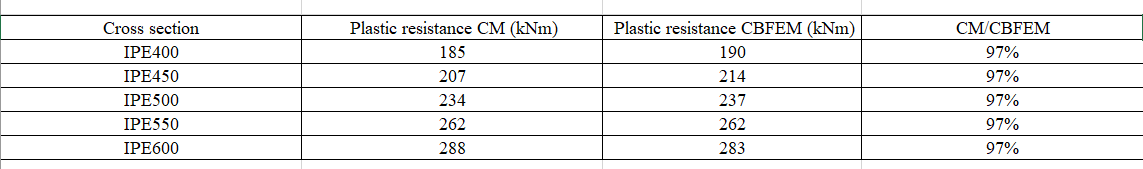
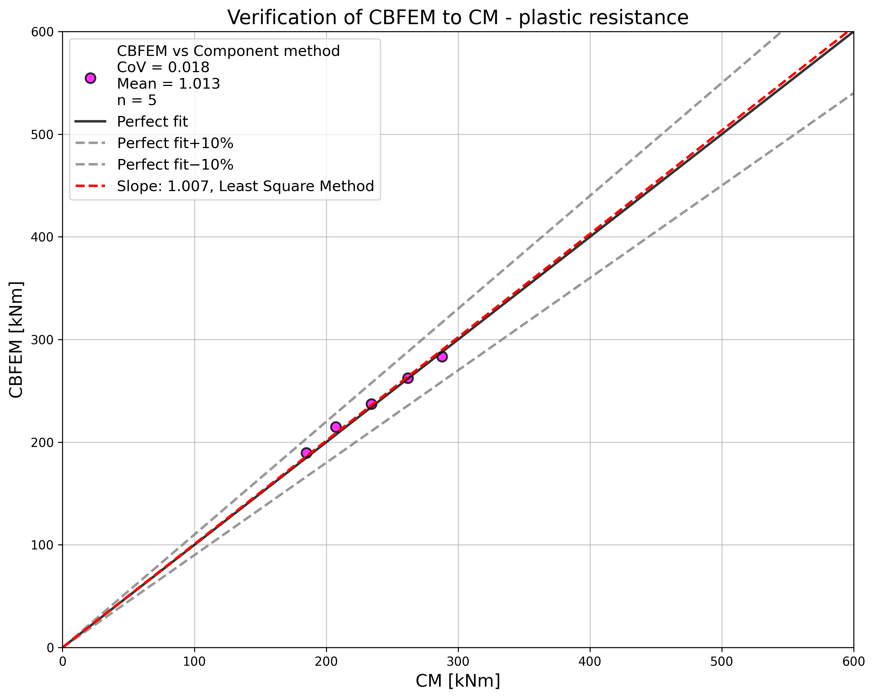
\[ \textsf{\textit{\footnotesize{Fig. 6.2.2a Verificarea CBFEM față de CM}}}\]

Tab. 6.2.2b Rezistența de calcul la flambaj

Tab. 6.2.2c Rezistențe la flambaj ale CM și CBFEM

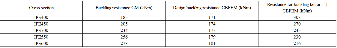
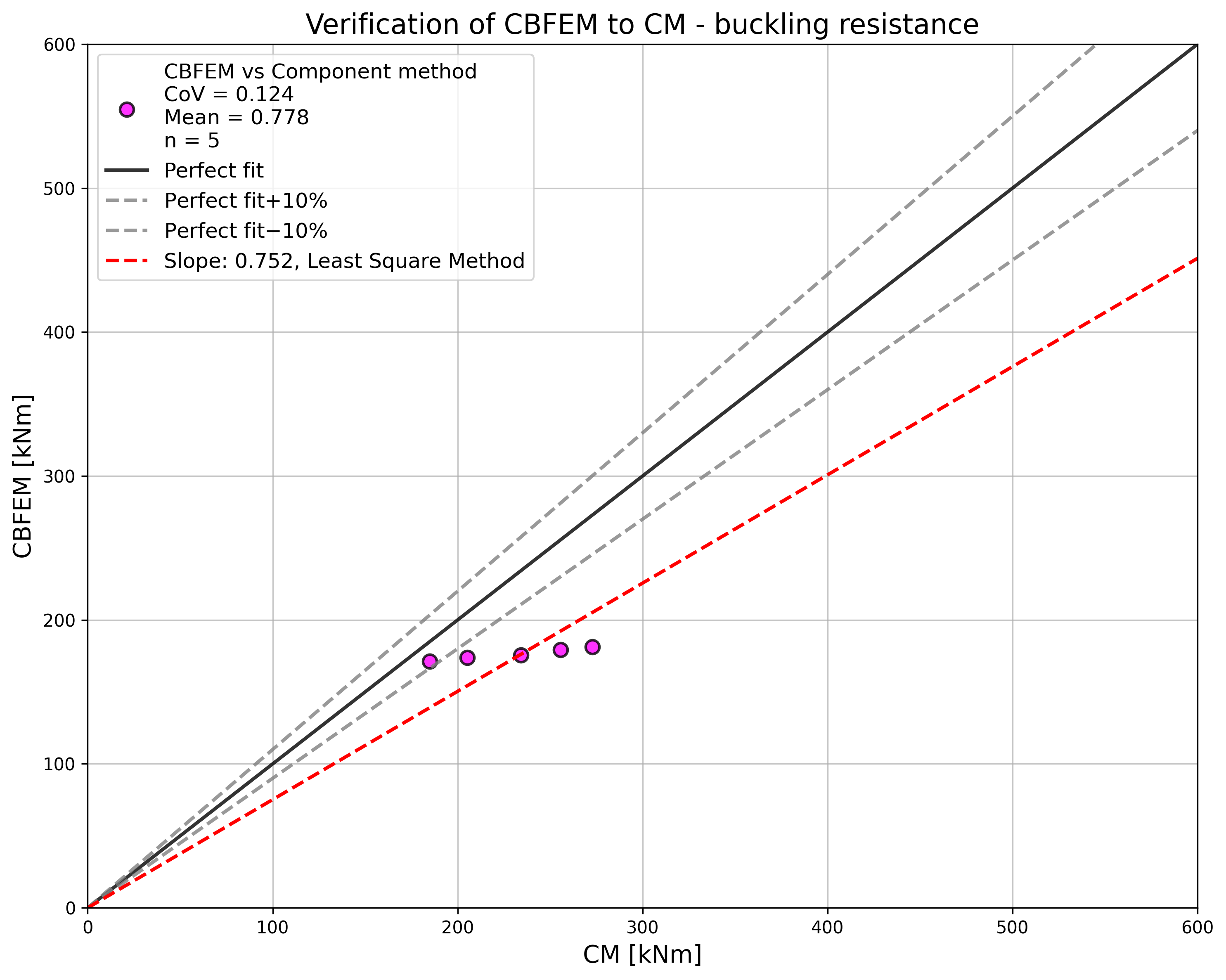
\[ \textsf{\textit{\footnotesize{Fig. 6.2.2c Verificarea CBFEM față de CM}}}\]

Rezultatele arată o bună concordanță în ceea ce privește sarcina critică și rezistența de calcul. Modelul CBFEM al îmbinării cu grinda IPE600 este prezentat în Fig. 6.2.3a. Primul mod de flambaj al îmbinării este prezentat în Fig. 6.2.3b.

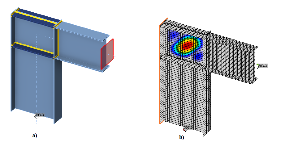
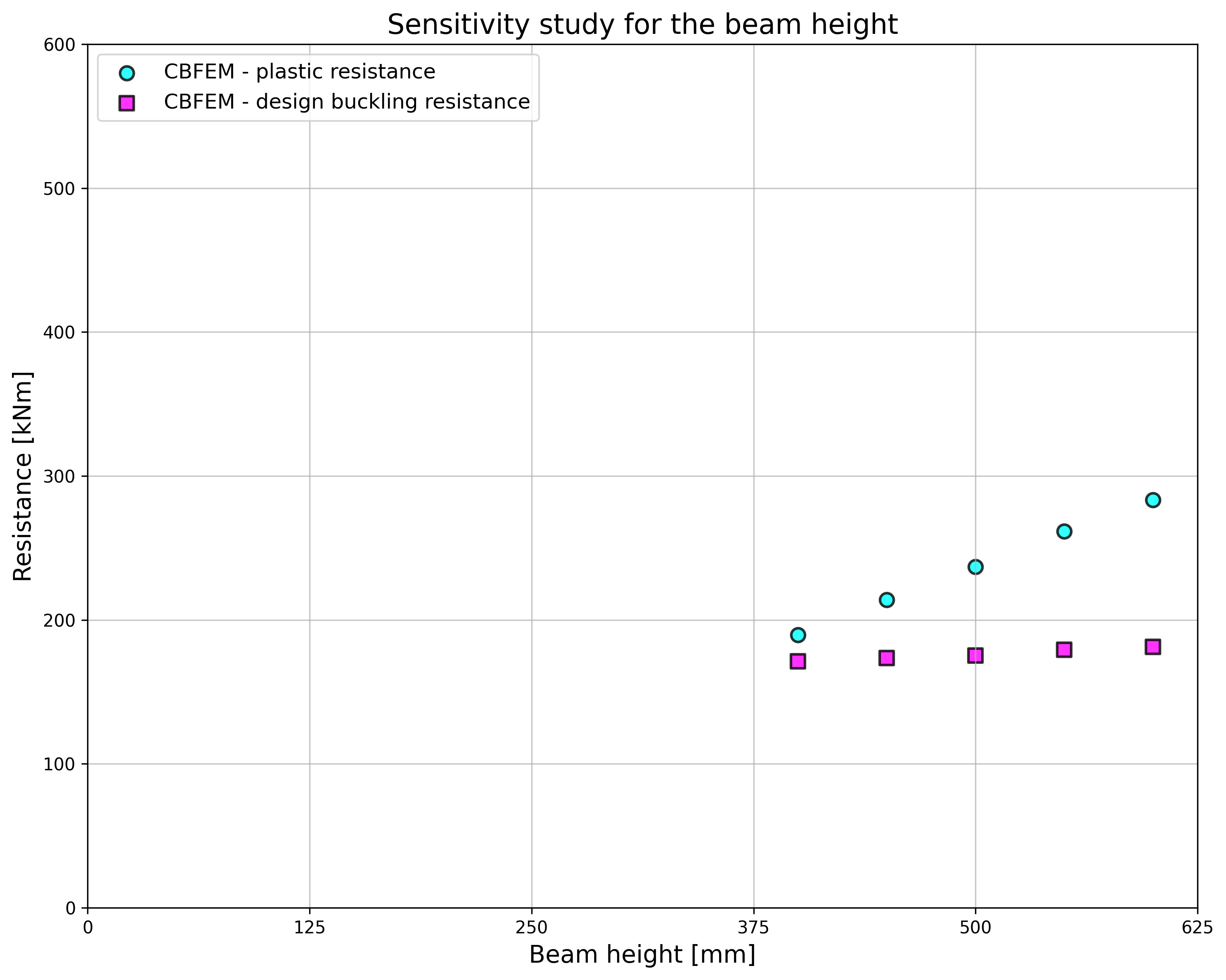
\[ \textsf{\textit{\footnotesize{c)}}}\]

\[ \textsf{\textit{\footnotesize{Fig. 6.2.3 a) Model CBFEM b) Primul mod de flambaj c) Influența înălțimii secțiunii transversale a grinzii asupra rezistențelor și sarcinilor critice}}}\]

Studiile de verificare au confirmat acuratețea modelului CBFEM pentru predicția comportamentului panoului inimii stâlpului. Rezultatele CBFEM sunt comparate cu rezultatele CM. Procedurile prevăd un comportament global similar al îmbinării.

Exemplu de referință

Date de intrare

Grindă

• Oțel S235
• IPE600

Stâlp

• Oțel S235
• Grosimea tălpii t_f = 10 mm
• Lățimea tălpii b_f = 250 mm
• Grosimea inimii t_w = 4 mm
• Înălțimea inimii h_w = 800 mm
• Înălțimea secțiunii h = 820 mm
• Depășire față de partea superioară a grinzii 20 mm

Element de rigidizare al inimii

• Oțel S235
• Grosimea elementului de rigidizare t_w = 19 mm
• Lățimea elementului de rigidizare h_w = 250 mm
• Suduri a_w,stiff = 10 mm
• Elemente de rigidizare opuse tălpii superioare și inferioare

Configurare cod – Model și plasă

• Numărul de elemente pe inima sau talpa celui mai mare element 24

Date de ieșire

• Sarcină la 5 % deformație plastică M_ult,k = 283 kNm
• Rezistența de calcul M_CBFEM = 181 kNm
• Factorul critic de flambaj (pentru M = 189 kNm) α_cr = 1,19
• Factorul de încărcare la 5 % deformație plastică α_ult,k = M_ult,k / M_CBFEM = 283/181 = 1,56

Referințe

EN 1993-1-5, Eurocode 3, Proiectarea structurilor de oțel – Partea 1-5: Elemente structurale din plăci, CEN, Bruxelles, 2005.

EN 1993-1-8, Eurocode 3, Proiectarea structurilor de oțel – Partea 1-8: Proiectarea îmbinărilor, CEN, Bruxelles, 2005.

Kuříková M., Wald F., Kabeláč J. Design of slender compressed plates in structural steel joints by component based finite element method, in SDSS 2019: International Colloquium on Stability and Ductility of Steel Structures, Prague, 2019.

Element de rigidizare a inimii stâlpului

Descriere

Obiectivul acestui studiu este verificarea metodei elementelor finite bazate pe componente (CBFEM) pentru un element de rigidizare a inimii stâlpului de clasa 4 într-o îmbinare grindă-stâlp, utilizând un model FEA de cercetare (RFEM) creat în software-ul Dlubal RFEM și metoda componentelor (CM).

Modelul FEA de cercetare

Modelul FEA de cercetare (RFEM) este utilizat pentru verificarea modelului CBFEM. În modelul numeric, se aplică elemente de tip coajă cvadrilaterale cu 4 noduri situate la colțuri. Se aplică analiza geometrică și material neliniară cu imperfecțiuni (GMNIA). Imperfecțiunile geometrice echivalente sunt derivate din primul mod de flambaj, iar amplitudinea este stabilită conform Anexei C din EN 1993-1-5:2006. Modelul numeric este prezentat în Fig. 6.3.1.

\[ \textsf{\textit{\footnotesize{Fig. 6.3.1 Modelul FEA de cercetare al unei îmbinări grindă-stâlp cu element de rigidizare zvelt al inimii stâlpului}}}\]

CBFEM

Procedura de calcul pentru plăci zvelte este descrisă în secțiunea 3.10. Analiza liniară de flambaj este implementată în software. Calculul rezistențelor de calcul se efectuează conform procedurii de calcul. F_CBFEM este interpolat de utilizator până când ρ ∙ α_ult,k/γ_M1 este egal cu 1. Se studiază o îmbinare grindă-stâlp cu un element de rigidizare zvelt al inimii stâlpului. Aceeași secțiune transversală este utilizată pentru grindă și stâlp. Grosimea elementului de rigidizare a inimii stâlpului variază. Geometria exemplelor este descrisă în Tab. 6.3.1. Îmbinarea este încărcată cu moment încovoietor.

Tab. 6.3.1 Prezentare generală a exemplelor

Exemplu	Talpă stâlp/grindă		Inimă stâlp/grindă		Element de rigidizare	Material
	bf	tf	hw	tw	ts
	[mm]	[mm]	[mm]	[mm]	[mm]
t3	400	20	600	12	3	S235
t4	400	20	600	12	4	S235
t5	400	20	600	12	5	S235
t6	400	20	600	12	6	S235

Comportament global și verificare

Comportamentul global al unei îmbinări grindă-stâlp cu un element de rigidizare zvelt al inimii stâlpului cu grosimea de 3 mm, descris prin diagrama moment-rotație în modelul CBFEM, este prezentat în Fig. 6.3.2. Atenția este concentrată asupra caracteristicilor principale: rezistența de calcul și sarcina critică. Diagrama este completată cu punctul în care începe curgerea și rezistența la 5% deformație plastică.

\[ \textsf{\textit{\footnotesize{Fig. 6.3.2 Curba moment-rotație pentru exemplul t3}}}\]

Verificarea rezistenței

Rezistența de calcul calculată cu software-ul CBFEM Idea StatiCa este comparată cu RFEM. Comparația este axată pe rezistența de calcul și sarcina critică. Rezultatele sunt prezentate în Tab. 6.3.2. Diagrama din Fig. 6.3.3 c) arată influența grosimii elementului de rigidizare a inimii stâlpului asupra rezistențelor și sarcinilor critice în exemplele examinate.

Tab. 6.3.2 Rezistențe de calcul și sarcini critice pentru RFEM și CBFEM

Rezultatele arată o concordanță foarte bună în ceea ce privește sarcina critică și rezistența de calcul. Modelul CBFEM al îmbinării cu element de rigidizare al inimii cu grosimea de 3 mm este prezentat în Fig. 6.3.3a. Primul mod de flambaj al îmbinării este prezentat în Fig. 6.3.3b.

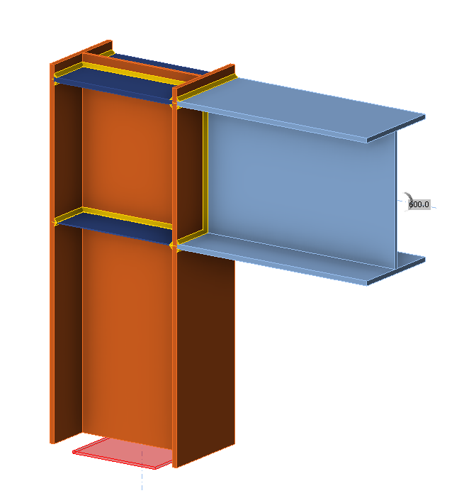
\[ \textsf{\textit{\footnotesize{a)}}}\]

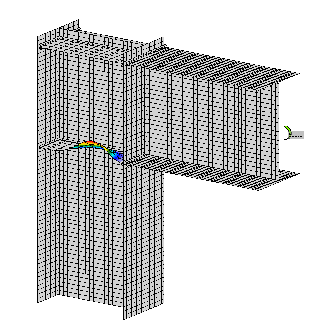
\[ \textsf{\textit{\footnotesize{b)}}}\]

\[ \textsf{\textit{\footnotesize{c)}}}\]

\[ \textsf{\textit{\footnotesize{Fig. 6.3.3 a) Model geometric b) Primul mod de flambaj c) Influența grosimii elementului de rigidizare asupra rezistențelor și sarcinilor critice}}}\]

Studiile de verificare au confirmat acuratețea modelului CBFEM pentru predicția comportamentului elementului de rigidizare a inimii stâlpului. Rezultatele CBFEM sunt comparate cu rezultatele RFEM. Toate procedurile prezic un comportament global similar al îmbinării. Diferența în rezistența de calcul este în toate cazurile sub 10%.

Exemplu de referință

Date de intrare

Grindă

• Oțel S235
• Grosimea tălpii t_f = 20 mm
• Lățimea tălpii b_f = 400 mm
• Grosimea inimii t_w = 12 mm
• Înălțimea inimii h_w = 600 mm

Stâlp

• Oțel S235
• Grosimea tălpii t_f = 20 mm
• Lățimea tălpii b_f = 400 mm
• Grosimea inimii t_w = 12 mm
• Înălțimea inimii h_w = 560 mm
• Înălțimea secțiunii h = 600 mm

Element de rigidizare superior al inimii stâlpului

• Oțel S235
• Grosimea elementului de rigidizare t_w = 20 mm
• Lățimea elementului de rigidizare h_w = 400 mm

Element de rigidizare inferior al inimii stâlpului

• Oțel S235
• Grosimea elementului de rigidizare t_w = 3 mm
• Lățimea elementului de rigidizare h_w = 400 mm

Configurare cod – Model și plasă

• Numărul de elemente pe inima sau talpa celui mai mare element 24

Rezultate

• Rezistența plastică CBFEM = 589 kNm
• Rezistența de calcul la flambaj CBFEM (kNm) = 309 kNm
• Factorul critic de flambaj (pentru rezistența de calcul la flambaj = 309 kNm) α_cr = 0,97
• Factorul de încărcare la 5% deformație plastică α_ult,k = Rezistența plastică CBFEM / Rezistența de calcul la flambaj CBFEM = 589/309 = 1,91

Noduri cu secțiuni tubulare

Secțiuni tubulare circulare

Metoda modurilor de cedare

În acest capitol, metoda elementelor finite bazată pe componente (CBFEM) pentru proiectarea îmbinărilor sudate uniplanare din Secțiuni Tubulare Circulare (CHS) este verificată față de Metoda Modurilor de Cedare (FMM): îmbinări T, X și K. În CBFEM, rezistența de calcul este limitată prin atingerea unei deformații de 5 % sau a unei forțe corespunzătoare unei deformații de 3% d₀ a îmbinării, unde d₀ este diametrul tălpii. Rezistența în FMM este determinată în general de sarcina maximă sau de limita de deformație de 3% d₀, vezi (Lu et al. 1994). FMM se bazează pe principiul identificării modurilor care pot cauza cedarea îmbinării. Din experiența practică și experimentele realizate în anii '70 și '80, au fost identificate două moduri de cedare pentru îmbinările CHS: plastificarea tălpii și forfecarea prin poansonare a tălpii. Această metodă de calcul este întotdeauna limitată la o geometrie verificată a îmbinărilor. Aceasta înseamnă că pentru fiecare geometrie se aplică întotdeauna formule diferite. În studiile următoare, sudurile sunt proiectate conform EN 1993‑1‑8:2006 pentru a nu fi componentele cele mai slabe ale îmbinării.

Plastificarea tălpii

Rezistența de calcul a feței tălpii unui profil CHS poate fi determinată folosind metoda dată de modelul FMM din Cap. 9 al prEN 1993-1-8:2020; vezi Fig. 7.1.1. Metoda este prezentată și în ISO/FDIS 14346 și este descrisă mai detaliat în (Wardenier et al. 2010). Rezistența de calcul a îmbinării CHS sudate încărcate axial este:

• pentru îmbinarea T și Y

\[ N_{1,Rd} = C_f \frac{f_{y0} t_0^2}{\sin{\theta_1}} (2.6+17.7 \beta^2) \gamma^{0.2} Q_f / \gamma_{M5} \]

• îmbinarea X

\[  N_{1,Rd} = C_f \frac{f_{y0} t_0^2}{\sin{\theta_1}} \left ( \frac{2.6+2.6 \beta}{1-0.7 \beta} \right ) \gamma^{0.15} Q_f / \gamma_{M5} \]

• și pentru îmbinarea K cu spațiu

\[ N_{1,Rd} = C_f \frac{f_{y0} t_0^2}{\sin{\theta_1}} (1.65+13.2 \beta^{1.6}) \gamma^{0.3} \left [ 1+ \frac{1}{1.2+(g/t_0)^{0.8}} \right ] Q_f / \gamma_{M5} \]

unde:           

• d_i – diametrul exterior al elementului CHS i (i = 0, 1, 2 sau 3)
• f_yi – limita de curgere a elementului i (i = 0, 1, 2 sau 3)
• g – spațiul dintre diagonalele îmbinării K
• t_i – grosimea peretelui elementului CHS i (i = 0, 1, 2 sau 3)
• \(\theta_i\) – unghiul dintre elementul diagonal i și talpă (i =1, 2 sau 3)
• \(\beta\) – raportul dintre diametrul mediu sau lățimea elementelor diagonale și cel al tălpii
• \(\gamma\) – raportul dintre lățimea sau diametrul tălpii și de două ori grosimea peretelui acesteia
• Q_f – factorul de tensiune al tălpii
• C_f – factorul de material
• \(\gamma_{M5}\) – factorul parțial de siguranță pentru rezistența îmbinărilor în grinzi cu zăbrele din secțiuni tubulare
• N_i,Rd – rezistența de calcul a unei îmbinări exprimată în termenii forței axiale interioare din elementul i (i = 0, 1, 2 sau 3)

\[ \textsf{\textit{\footnotesize{Fig. 7.1.1 Modul de cedare examinat – plastificarea tălpii}}}\]

Forfecarea prin poansonare a tălpii

(pentru \(d_i \le d_0 - 2 t_0\))

Rezistența de calcul a îmbinării T, Y, X și K sudate din secțiuni tubulare circulare, încărcate axial, la forfecarea prin poansonare a tălpii (Fig. 7.1.2) este:

\[ N_{1,Rd} = C_f \frac{f_{y0}}{\sqrt{3}} t_0 \pi d_i \frac{1+\sin{\theta_1}}{2 \sin^2{\theta_1}} / \gamma_{M5} \]

unde:

• d_i – diametrul exterior al elementului CHS i (i = 0,1,2 sau 3)
• t_i – grosimea peretelui elementului CHS i (i = 0,1,2 sau 3)
•  f_y,i – limita de curgere a elementului i (i = 0,1,2 sau 3)
• \(\theta_i\) – unghiul dintre elementul diagonal i și talpă (i = 1,2 sau 3)
• C_f – factorul de material
• N_i,Rd – rezistența de calcul a unei îmbinări exprimată în termenii forței axiale interioare din elementul i (i = 0, 1, 2 sau 3)

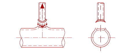
\[ \textsf{\textit{\footnotesize{Fig. 7.1.2 Modul de cedare examinat – forfecarea prin poansonare a tălpii}}}\]

Forfecarea tălpii

(pentru îmbinările X, numai dacă \(\cos{\theta_1} > \beta\))

Rezistența de calcul a îmbinării X sudate din secțiuni tubulare circulare, încărcate axial, la forfecarea tălpii, vezi Fig. 7.1.3, este:

\[ N_{1,Rd} = \frac{f_{y0}}{\sqrt{3}} \frac{(2/\pi A_0)}{\sin{\theta_1}} / \gamma_{M5} \]

unde:

• A_i – aria secțiunii transversale i (i = 0,1,2 sau 3)
• f_y,i – limita de curgere a elementului i (i = 0,1,2 sau 3)
• \(\theta_i\) – unghiul dintre elementul diagonal i și talpă (i = 1,2 sau 3)
• N_i,Rd – rezistența de calcul a unei îmbinări exprimată în termenii forței axiale interioare din elementul i (i = 0, 1, 2 sau 3)

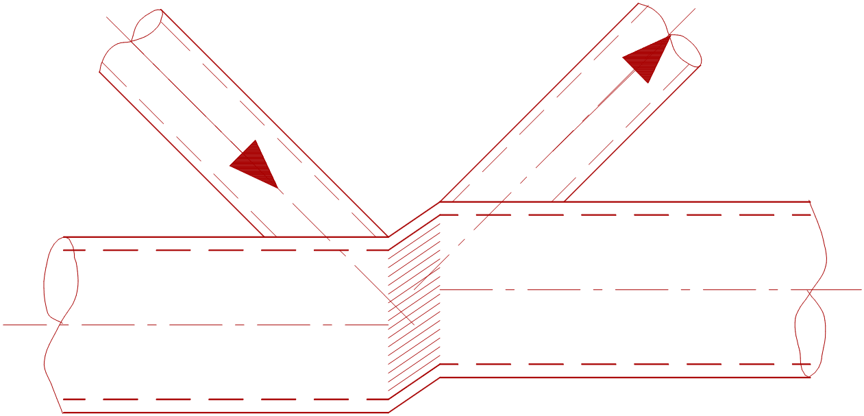
\[ \textsf{\textit{\footnotesize{Fig. 7.1.3 Modul de cedare examinat - Forfecarea tălpii}}}\]

Domeniu de valabilitate

CBFEM a fost verificat pentru îmbinări tipice din secțiuni tubulare circulare sudate. Domeniul de valabilitate pentru aceste îmbinări este definit în Tabelul 7.1.8 din prEN 1993-1-8:2020; vezi Tab. 7.1.2. Același domeniu de valabilitate se aplică modelului CBFEM. În afara domeniului de valabilitate al FMM, trebuie pregătit un experiment pentru validare sau efectuată o verificare conform unui model de cercetare validat.

Tab. 7.1.2 Domeniu de valabilitate pentru metoda modurilor de cedare

General	\(0.2 \le \frac{d_i}{d_0} \le 1.0 \)	\( \theta_i \ge 30^{\circ} \)	\(-0.55 \le \frac{e}{d_0} \le 0.25 \)
	\(g \ge t_1+t_2 \)	\(f_{yi} \le f_{y0} \)	\( t_i \le t_0 \)

Talpă	Compresiune	Clasa 1 sau 2 și \(10 \le d_0 / t_0 \le 50 \) (dar pentru îmbinările X: \( d_0/t_0 \le 40 \))
	Întindere	\(10 \le d_0 / t_0 \le 50 \) (dar pentru îmbinările X: \( d_0/t_0 \le 40 \))
Diagonale CHS	Compresiune	Clasa 1 sau 2 și \(d_i / t_i \le 50\)
	Întindere	\(d_i / t_i \le 50 \)

Îmbinare uniplanară T și Y-CHS

O prezentare generală a exemplelor considerate în studiu este dată în Tab. 7.1.3. Cazurile selectate acoperă o gamă largă de rapoarte geometrice ale îmbinărilor. Geometria îmbinărilor cu dimensiuni este prezentată în Fig. 7.1.2. În cazurile selectate, îmbinările au cedat conform FMM prin plastificarea tălpii sau forfecarea prin poansonare.

\[ \textsf{\textit{\footnotesize{Fig. 7.1.4 Dimensiunile îmbinării T/Y}}}\]

Tab. 7.1.3 Prezentare generală a exemplelor

Exemplu	Talpă	Diagonală	Unghiuri		Material
	Secțiune	Secțiune	\(\theta\)	fy	fu	E
			[°]	[MPa]	[MPa]	[GPa]
1	CHS219.1/5.0	CHS48.3/5.0	90	355	490	210
2	CHS219.1/5.0	CHS114.3/6.3	90	355	490	210
3	CHS219.1/6.3	CHS114.3/6.3	90	355	490	210
4	CHS219.1/10.0	CHS60.3/5.0	90	355	490	210
5	CHS219.1/12.5	CHS168.3/10.0	90	355	490	210
6	CHS219.1/8.0	CHS48.3/5.0	90	355	490	210

Verificarea rezistenței

Rezultatele metodei bazate pe FMM sunt comparate cu rezultatele CBFEM. Comparația este axată pe rezistență și modul de cedare de calcul. Rezultatele sunt prezentate în Tab. 7.1.4.

Studiul arată o bună concordanță pentru cazurile de încărcare aplicate. Rezultatele sunt rezumate într-o diagramă care compară rezistențele de calcul ale CBFEM și FMM; vezi Fig. 7.1.5. Rezultatele arată că diferența dintre cele două metode de calcul este în toate cazurile mai mică de 14%.

Tab. 7.1.4 Compararea rezistențelor de calcul pentru încărcare la întindere/compresiune: predicție prin CBFEM și FMM

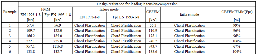
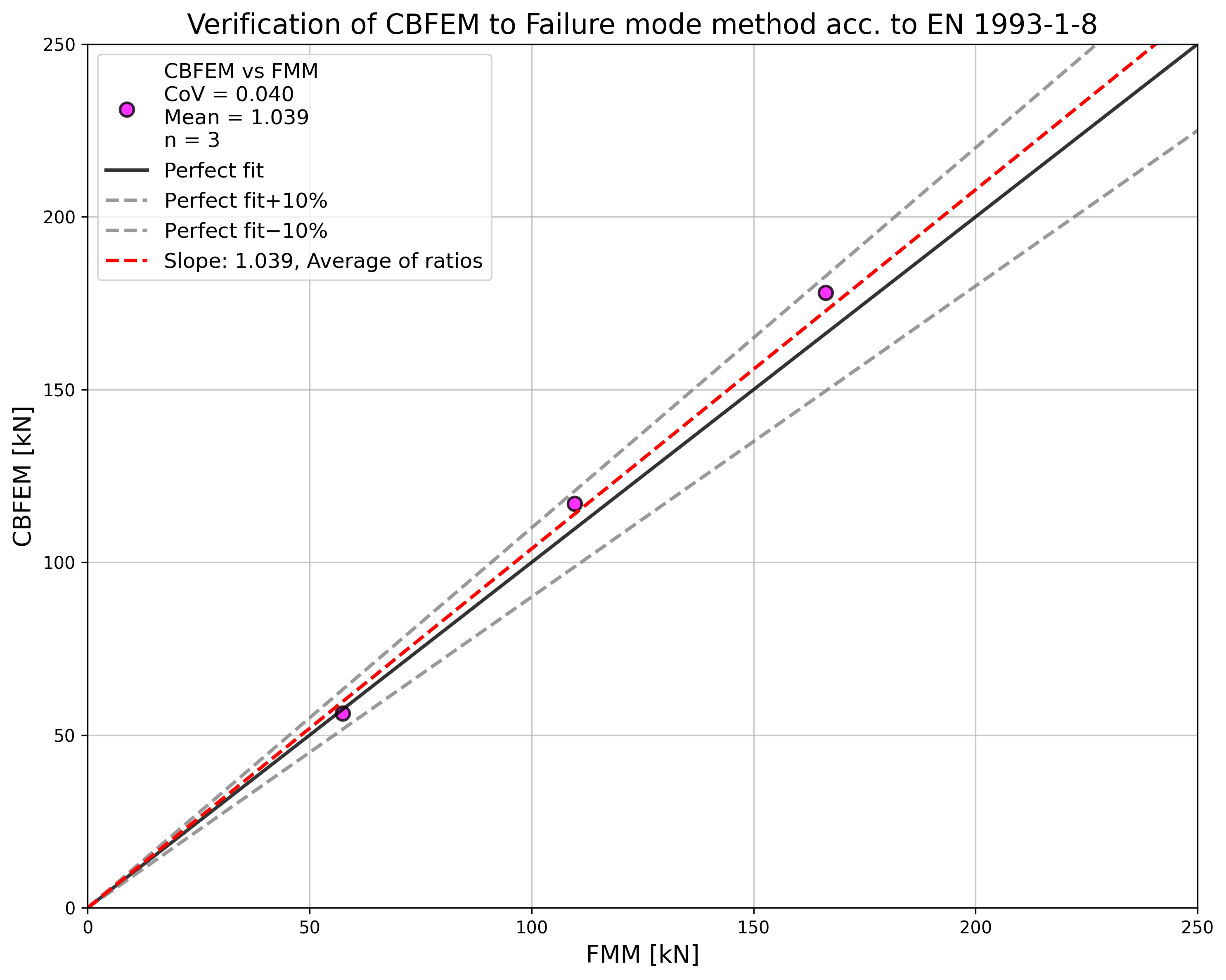
\[ \textsf{\textit{\footnotesize{Fig. 7.1.5 Verificarea CBFEM față de EN 1993-1-8 pentru îmbinarea uniplanară CHS T și Y}}}\]

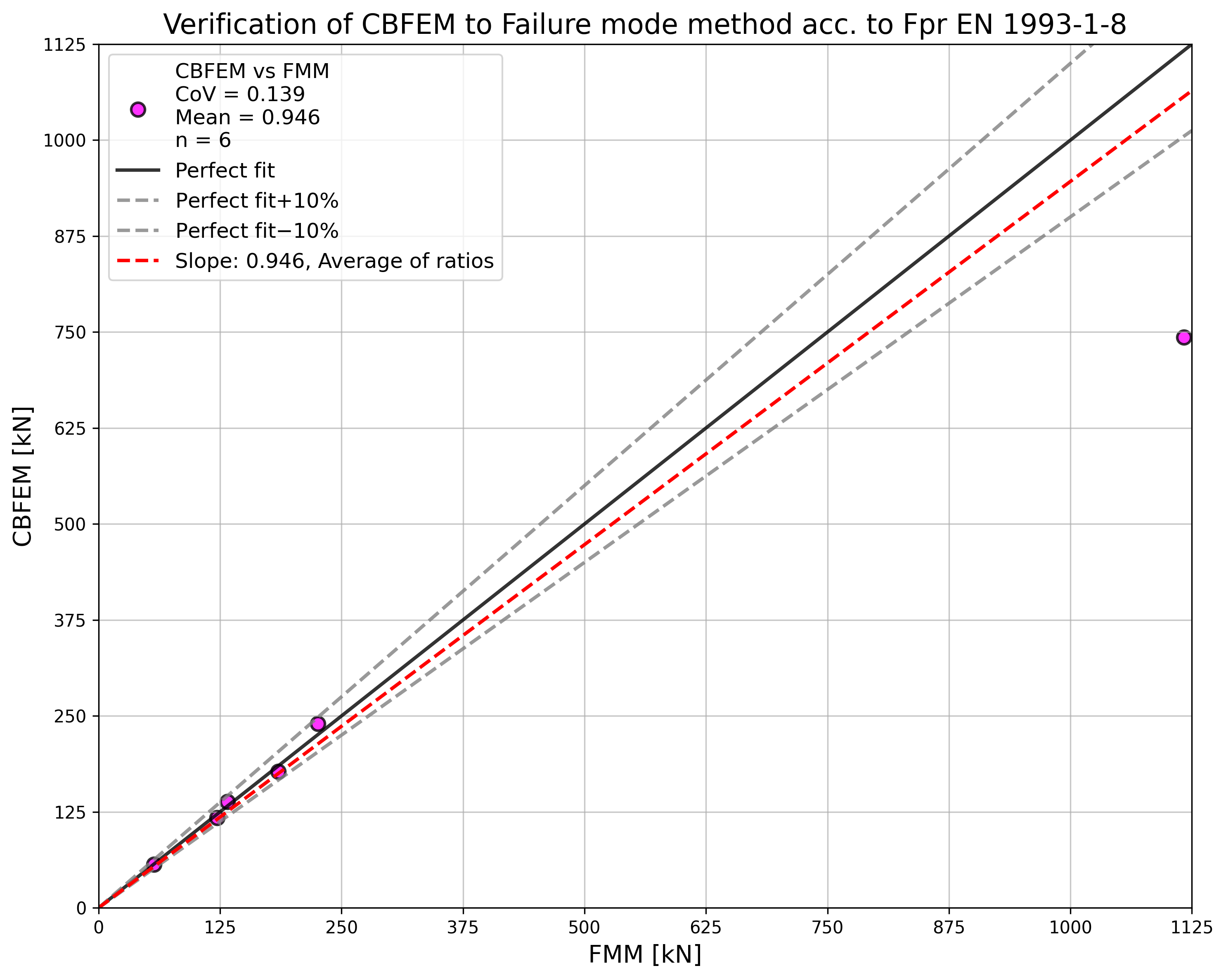
\[ \textsf{\textit{\footnotesize{Fig. 7.1.6 Verificarea CBFEM față de Fpr EN 1993-1-8 pentru îmbinarea uniplanară CHS T și Y}}}\]

Exemplu de referință

Date de intrare

Talpă

• Oțel S355
• Secțiune CHS219.1/5.0

Diagonală

• Oțel S355
• Secțiune CHS48.3/5.0
• Unghi dintre elementul diagonal și talpă 90°

Sudură

• Sudură cap la cap în jurul diagonalei

Încărcare

• Prin forță aplicată diagonalei la compresiune

Dimensiunea plasei

• 64 elemente de-a lungul suprafeței elementului tubular circular

Rezultate

• Rezistența de calcul la compresiune este N_Rd = 56,3 kN
• Modul de cedare de calcul este plastificarea tălpii

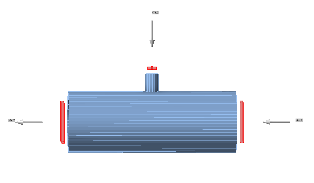
\[ \textsf{\textit{\footnotesize{Fig. 7.1.6a Condiții la limită pentru îmbinarea uniplanară CHS T și Y}}}\]

Îmbinare uniplanară X-CHS

O prezentare generală a exemplelor considerate în studiu este dată în Tab. 7.1.5. Cazurile selectate acoperă o gamă largă de rapoarte geometrice ale îmbinărilor. Geometria îmbinărilor cu dimensiuni este prezentată în Fig. 7.1.6. În cazurile selectate, îmbinările au cedat conform FMM prin plastificarea tălpii sau forfecarea prin poansonare.

\[ \textsf{\textit{\footnotesize{Fig. 7.1.7 Dimensiunile îmbinării X}}}\]

Tab. 7.1.5 Prezentare generală a exemplelor

Exemplu	Talpă	Diagonală	Unghiuri		Material
	Secțiune	Secțiune	\(\theta\)	fy	fu	E
			[°]	[MPa]	[MPa]	[GPa]
1	CHS219.1/6.3	CHS60.3/5.0	90	355	490	210
2	CHS219.1/8.0	CHS76.1/5.0	90	355	490	210
3	CHS219.1/10.0	CHS139.7/10.0	90	355	490	210
4	CHS219.1/12.5	CHS114.3/6.3	90	355	490	210
5	CHS219.1/10.0	CHS76.1/5.0	90	355	490	210
6	CHS219.1/8.0	CHS114.3/6.3	90	355	490	210
7	CHS219.1/6.3	CHS48.3/5.0	60	355	490	210
8	CHS219.1/6.3	CHS114.3/6.3	60	355	490	210
9	CHS219.1/8.0	CHS60.3/5.0	60	355	490	210
10	CHS219.1/10.0	CHS114.3/6.3	60	355	490	210
11	CHS219.1/12.5	CHS139.7/10.0	60	355	490	210
12	CHS219.1/8.0	CHS139.7/10.0	60	355	490	210
13	CHS219.1/6.3	CHS48.3/5.0	30	355	490	210
14	CHS219.1/6.3	CHS193.7/12.5	30	355	490	210
15	CHS219.1/6.3	CHS219.1/12.5	30	355	490	210
16	CHS219.1/8.0	CHS76.1/5.0	30	355	490	210
17	CHS219.1/8.0	CHS168.3/10	30	355	490	210
18	CHS219.1/12.5	CHS168.3/10	30	355	490	210

Verificarea rezistenței

Rezultatele CBFEM sunt comparate cu rezultatele FMM. Comparația este axată pe rezistență și modul de cedare de calcul. Rezultatele sunt prezentate în Tab. 7.1.6.

Tab. 7.1.6 Compararea rezultatelor predicției prin CBFEM și FMM

Studiul arată o bună concordanță pentru majoritatea cazurilor de încărcare aplicate. Rezultatele sunt rezumate într-o diagramă care compară rezistențele de calcul ale CBFEM și FMM; vezi Fig. 7.1.7. Rezultatele arată că diferența dintre cele două metode de calcul este în majoritatea cazurilor mai mică de 13%. 

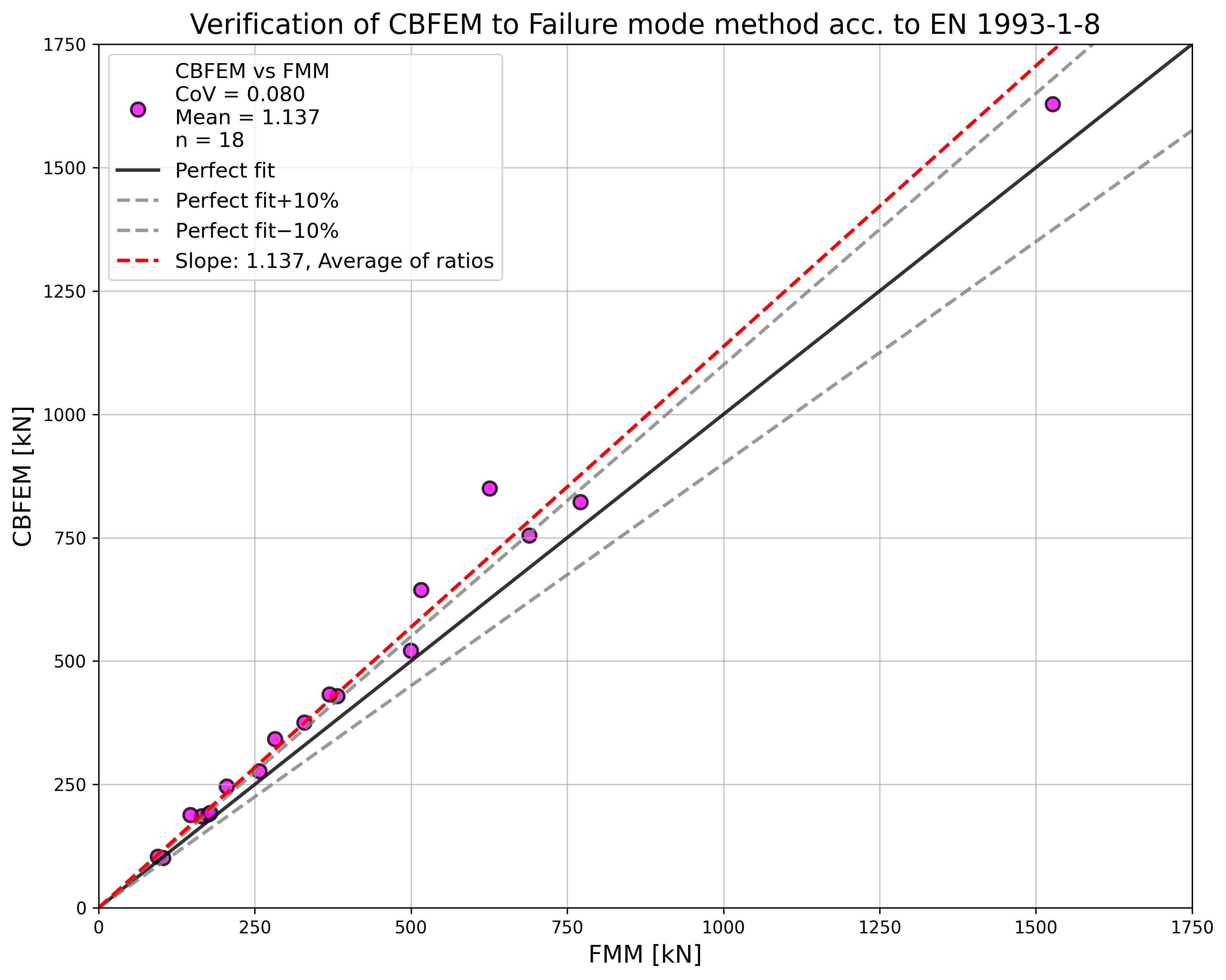
\[ \textsf{\textit{\footnotesize{Fig. 7.1.8 Verificarea CBFEM față de EN 1993-1-8 pentru îmbinarea uniplanară CHS X}}}\]

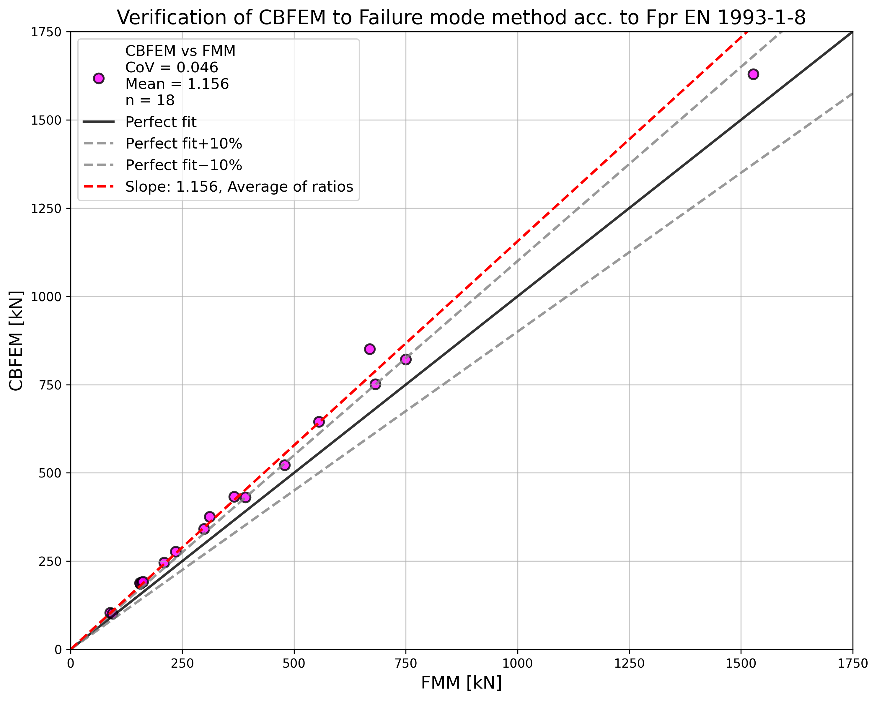
\[ \textsf{\textit{\footnotesize{Fig. 7.1.9 Verificarea CBFEM față de Fpr EN 1993-1-8 pentru îmbinarea uniplanară CHS X}}}\]

Exemplu de referință

Date de intrare

Talpă

• Oțel S355
• Secțiune CHS219.1/6,3

Diagonală

• Oțel S355
• Secțiune CHS60,3/5,0
• Unghi dintre elementul diagonal și talpă 90°

Sudură

• Sudură cap la cap în jurul diagonalei

Încărcare

• Prin forță aplicată diagonalei la compresiune

Dimensiunea plasei

• 64 elemente de-a lungul suprafeței elementului tubular circular

Rezultate

• Rezistența de calcul la compresiune este N_Rd = 103,9 kN
• Modul de cedare de calcul este plastificarea tălpii

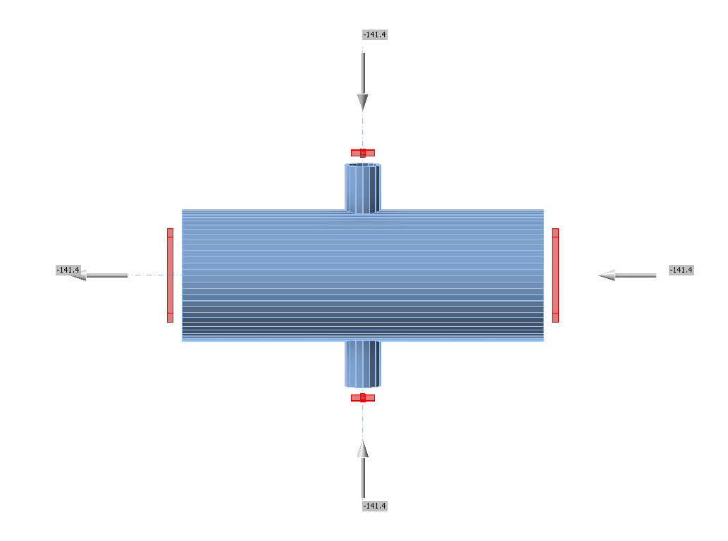
\[ \textsf{\textit{\footnotesize{Fig. 7.1.9a Condiții la limită pentru îmbinarea uniplanară CHS X}}}\]

Îmbinare uniplanară K-CHS

O prezentare generală a exemplelor considerate în studiu este dată în Tab. 7.1.7. Cazurile selectate acoperă o gamă largă de rapoarte geometrice ale îmbinărilor. Geometria îmbinărilor cu dimensiuni este prezentată în Fig. 7.1.8. În cazurile selectate, îmbinările au cedat conform metodei bazate pe modurile de cedare (FMM) prin plastificarea tălpii sau forfecarea prin poansonare.

Tab. 7.1.7 Prezentare generală a exemplelor

Exemplu	Talpă	Diagonală	Spațiu	Unghiuri		Material
	Secțiune	Secțiune	g	\(\theta\)	fy	fu	E
			[mm]	[°]	[MPa]	[MPa]	[GPa]
1	CHS219,1/8,0	CHS88,9/5,0	23.8	60	355	490	210
2	CHS219,1/12,5	CHS88,9/5,0	23.8	60	355	490	210
3	CHS219,1/5,0	CHS88,9/5,0	23.8	60	355	490	210
4	CHS219,1/10,0	CHS60,3/5,0	56.9	60	355	490	210
5	CHS219,1/6,3	CHS88,9/5,0	23.8	60	355	490	210
6	CHS219,1/6,3	CHS60,3/5,0	56.9	60	355	490	210
7	CHS219,1/8,0	CHS76,1/5,0	38.6	60	355	490	210
8	CHS219,1/10,0	CHS76,1/5,0	38.6	60	355	490	210
9	CHS219,1/6.3	CHS48,3/65,0	70.7	60	355	490	210
10	CHS219,1/12,5	CHS48,3/5,0	70.7	60	355	490	210

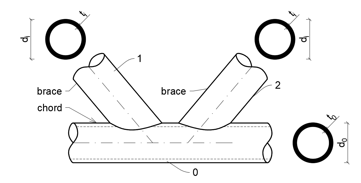
\[ \textsf{\textit{\footnotesize{Fig. 7.1.10 Dimensiunile îmbinării K}}}\]

Verificarea rezistenței

Rezultatele metodei bazate pe modurile de cedare (FMM) sunt comparate cu rezultatele CBFEM. Comparația este axată pe rezistență și modul de cedare de calcul. Rezultatele sunt prezentate în Tab. 7.1.8 și în Fig. 7.1.9.

Tab. 7.1.8 Compararea rezultatelor rezistențelor de calcul prin CBFEM și FMM

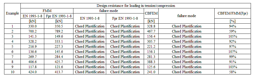
Studiul arată o bună concordanță pentru cazurile de încărcare aplicate. Rezultatele sunt rezumate într-o diagramă care compară rezistențele de calcul ale CBFEM și FMM; vezi Fig. 7.1.6. Rezultatele arată că diferența dintre cele două metode de calcul este în toate cazurile mai mică de 12 %.

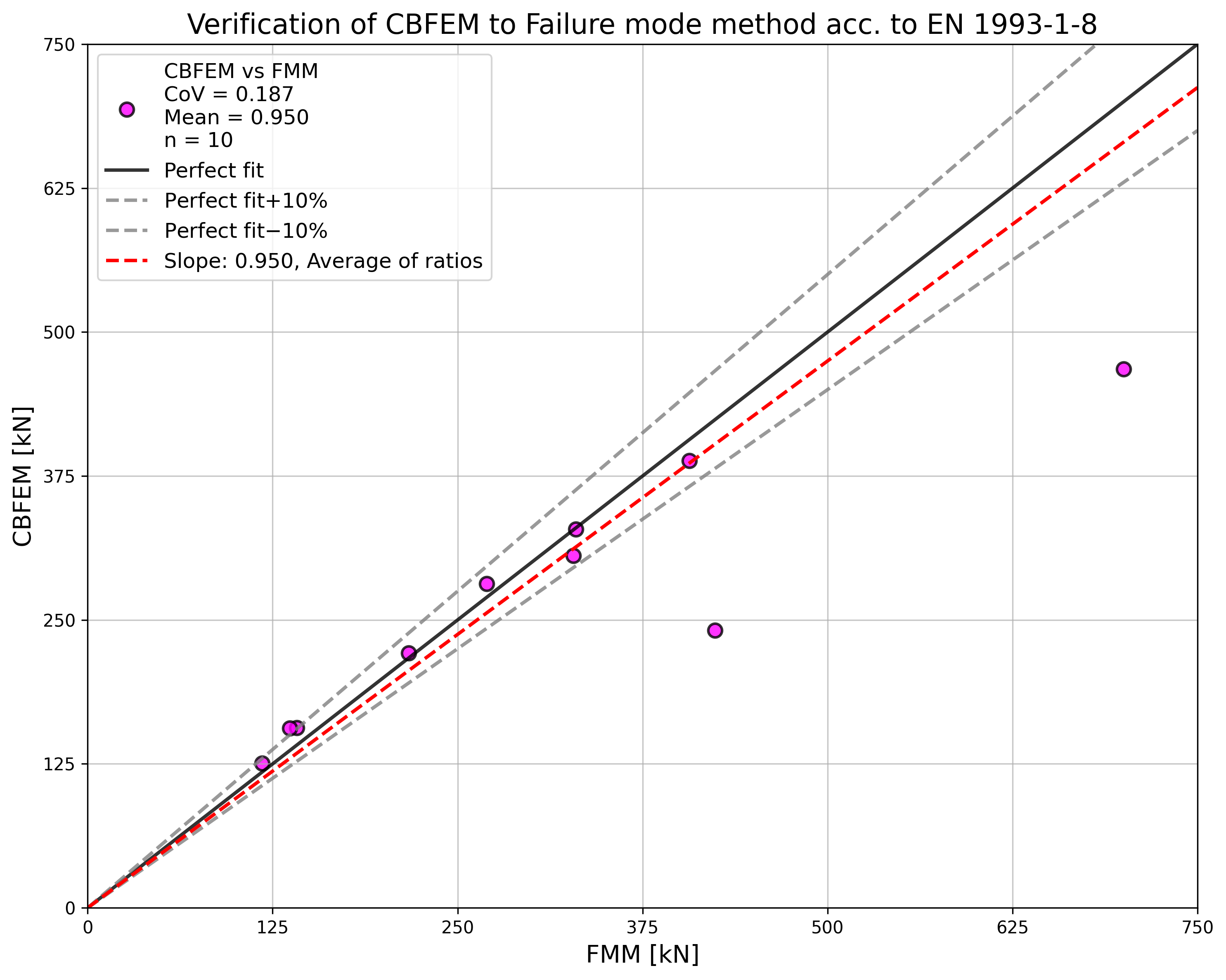
\[ \textsf{\textit{\footnotesize{Fig. 7.1.11 Verificarea CBFEM față de EN 1993-1-8 pentru îmbinarea uniplanară CHS K}}}\]

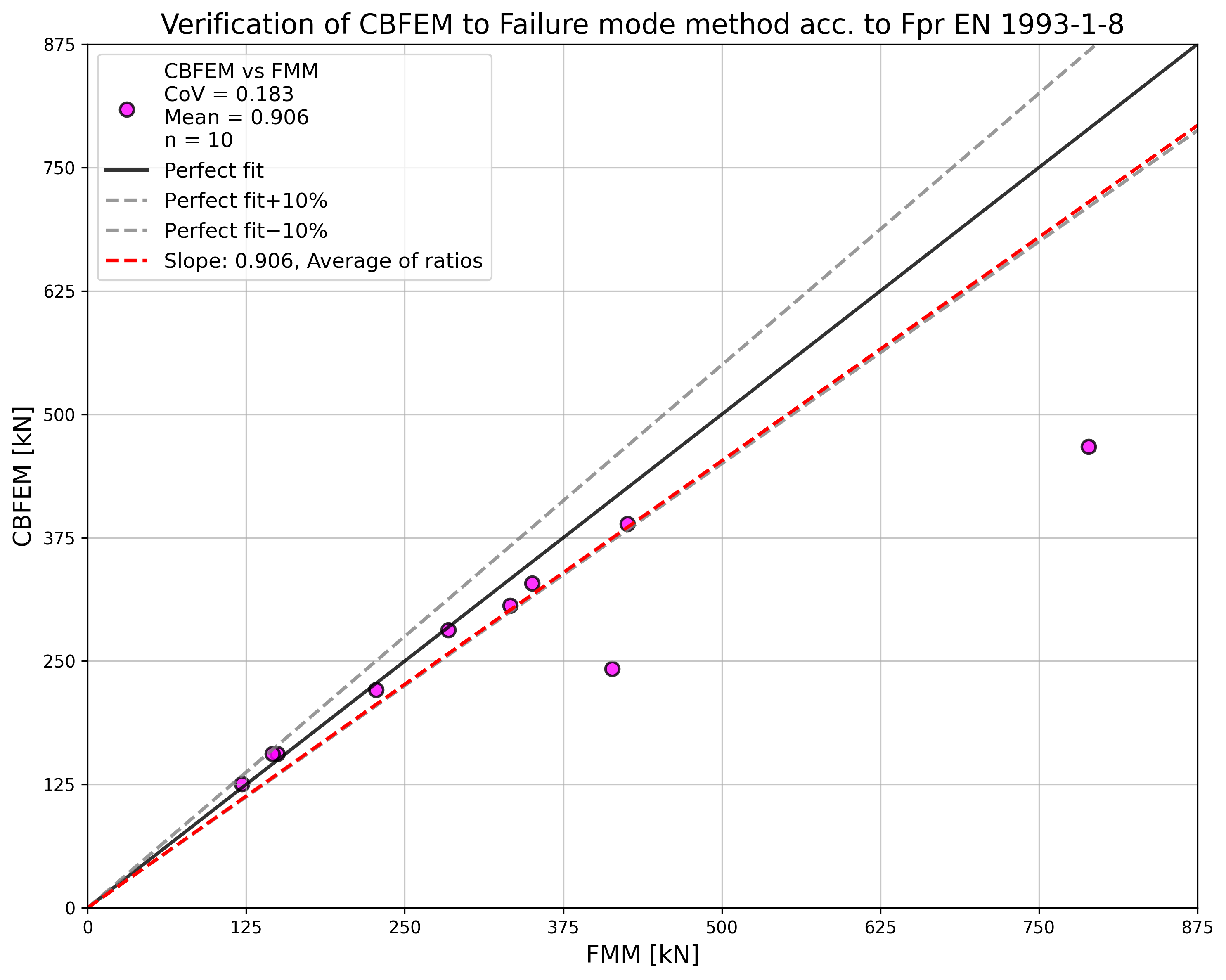
\[ \textsf{\textit{\footnotesize{Fig. 7.1.12 Verificarea CBFEM față de Fpr EN 1993-1-8 pentru îmbinarea uniplanară CHS K}}}\]

Exemplu de referință

Date de intrare

Talpă

• Oțel S355
• Secțiune CHS 219.1/8.0

Diagonală

• Oțel S355
• Secțiune CHS 88.9/5.0
• Unghi dintre elementul diagonal și talpă 60°
• Spațiu dintre diagonale g = 23,8 mm

Sudură

• Sudură cap la cap în jurul diagonalei

Încărcare

• Prin forță aplicată diagonalei la compresiune

Dimensiunea plasei

• 64 elemente de-a lungul suprafeței elementului tubular circular

Rezultate

• Rezistența de calcul la compresiune este N_Rd = 328,8 kN
• Modul de cedare de calcul este plastificarea tălpii

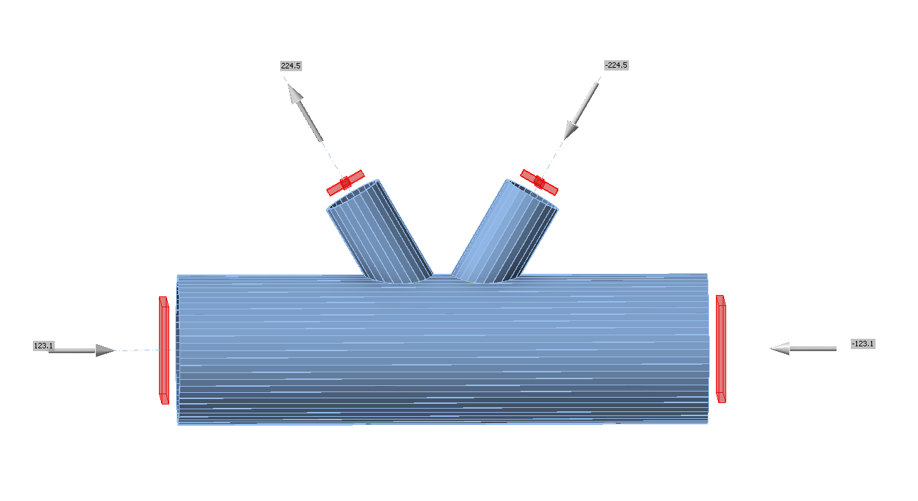
\[ \textsf{\textit{\footnotesize{Fig. 7.1.6a Condiții la limită pentru îmbinarea uniplanară CHS K}}}\]

Secțiuni tubulare dreptunghiulare

Descriere

În acest capitol, îmbinările T, X și K cu rost sudate uniplanare din secțiuni tubulare dreptunghiulare și pătrate, prevăzute prin CBFEM, sunt verificate. Diagonala din secțiune tubulară pătrată (SHS) este sudată direct pe talpa RHS fără utilizarea plăcilor de ranforsare. Îmbinările sunt încărcate cu forță axială. În CBFEM, rezistența de calcul este limitată la 5 % deformație sau la o forță corespunzătoare deformației de 0,03b₀ a îmbinării, iar în FMM în general prin deformația din plan a plăcii de 0,03b₀, unde b₀ este înălțimea tălpii RHS; a se vedea Lu et al. (1994).

Metoda modurilor de cedare

În cazul îmbinărilor T, Y, X sau K cu rost încărcate axial din secțiuni tubulare dreptunghiulare sudate, pot apărea cinci moduri de cedare. Acestea sunt: cedarea feței tălpii, plastificarea tălpii, cedarea peretelui lateral al tălpii, cedarea inimii tălpii, cedarea la forfecare a tălpii, cedarea la forfecare prin perforare și cedarea diagonalei. În acest studiu, cedarea feței tălpii, cedarea diagonalei și cedarea la forfecare prin perforare sunt examinate pentru îmbinările T, Y și X, iar cedarea feței tălpii, cedarea la forfecare a tălpii, cedarea diagonalei și cedarea la forfecare prin perforare sunt examinate pentru îmbinarea K cu rost; a se vedea Fig. 7.2.1. Sudurile proiectate conform EN 1993-1-8:2005 nu reprezintă componentele cele mai slabe ale îmbinării.

\[ \textsf{\textit{\footnotesize{Fig. 7.2.1 Moduri de cedare examinate: a) Cedarea feței tălpii, b) Cedarea la forfecare a tălpii, c) Cedarea diagonalei și d) Cedarea la forfecare prin perforare}}}\]

Cedarea feței tălpii

Rezistența de calcul a feței tălpii RHS este determinată prin modelul FMM din secțiunea 9.5 a EN 1993‑1-8:2020. Metoda este prezentată și în ISO/FDIS 14346 și este descrisă în detaliu în Wardenier et al. (2010). Rezistența de calcul a îmbinării T, Y sau X încărcate axial din secțiuni tubulare dreptunghiulare sudate este

\[ N_{i,Rd} = C_f \frac{f_{y0} t_0^2}{\sin{\theta_i}} \left ( \frac{2 \eta}{(1-\beta) \sin{\theta_i}} + \frac{4}{\sqrt{1-\beta}} \right ) Q_f / \gamma_{M5} \]

Rezistența de calcul a îmbinării K cu rost încărcate axial din secțiuni tubulare dreptunghiulare sudate este

\[ N_{i,Rd} = 8.9 C_f \beta \gamma^{0.5} \frac{f_{y,0} t_0^2}{\sin{\theta_i}} Q_f / \gamma_{M5} \]

unde C_f este factorul de material, f_y0 este limita de curgere a tălpii, t₀ este grosimea peretelui tălpii, η este raportul dintre înălțimea diagonalei și lățimea tălpii, β este raportul dintre lățimea diagonalei și lățimea tălpii, q_i este unghiul dintre diagonala i și talpă (i = 1, 2), Q_f este funcția de tensiune a tălpii, iar γ este raportul de zveltețe al tălpii.

Cedarea diagonalei

Rezistența de calcul a feței tălpii RHS poate fi determinată folosind metoda dată de modelul FMM din secțiunea 9.5 a EN 1993-1-8:2020. Rezistența de calcul a îmbinării T, Y sau X încărcate axial din secțiuni tubulare dreptunghiulare sudate este

\[ N_{i,Rd} = C_f f_{yi} t_i (2 h_i - 4 t_i + 2 b_{eff} ) / \gamma_{M5} \]

Rezistența de calcul a îmbinării K cu rost încărcate axial din secțiuni tubulare dreptunghiulare sudate este

\[ N_{i,Rd} = C_f f_{yi} t_i (2 h_i - 4 t_i + b_i + b_{eff} ) / \gamma_{M5} \]

unde C_f este factorul de material, f_yi este limita de curgere a diagonalei i (i = 1, 2), t_i este grosimea peretelui diagonalei i, h_i este înălțimea diagonalei i, b_i este lățimea diagonalei i, b_eff este lățimea efectivă a diagonalei.

Forfecare prin perforare

Rezistența de calcul a îmbinării T, Y sau X încărcate axial din secțiuni tubulare dreptunghiulare sudate este

\[ N_{i,Rd} = C_f \frac{f_{y0} t_0}{\sqrt{3}\sin{\theta_i}} \left( \frac{2h_i}{\sin{\theta_i}} + 2b_{e,p} \right ) / \gamma_{M5} \]

Rezistența de calcul a îmbinării K cu rost încărcate axial din secțiuni tubulare dreptunghiulare sudate este

\[ N_{i,Rd} = C_f \frac{f_{y0} t_0}{\sqrt{3}\sin{\theta_i}} \left( \frac{2h_i}{\sin{\theta_i}} + b_i+b_{e,p} \right ) / \gamma_{M5} \]

Unde C_f este factorul de material, f_y0 este limita de curgere a tălpii, t₀ este grosimea peretelui tălpii, q_i este unghiul dintre diagonala i și talpă (i = 1, 2), h_i este înălțimea diagonalei i, b_i este lățimea diagonalei i și b_e,p este lățimea efectivă pentru forfecarea prin perforare.

Cedarea la forfecare a tălpii

Rezistența de calcul a îmbinării K cu rost încărcate axial din secțiuni tubulare dreptunghiulare sudate este

\[ N_{i,Rd} = \frac{f_{y0}A_{V,0,gap}}{\sqrt{3}\sin{\theta_i}}/\gamma_{M5} \]

unde f_y0 este limita de curgere a tălpii, A_v,0,gap este aria efectivă pentru cedarea la forfecare a tălpii, iar q_i este unghiul dintre diagonala i și talpă (i = 1, 2).

Domeniu de valabilitate

CBFEM a fost verificat pentru îmbinările tipice T, Y, X și K cu rost din secțiuni tubulare dreptunghiulare sudate. Domeniul de valabilitate pentru aceste îmbinări este definit în Tabelul 9.2 din prEN 1993-1-8:2020; a se vedea Tab. 7.2.1. Același domeniu de valabilitate se aplică modelului CBFEM. În afara domeniului de valabilitate al FMM, trebuie pregătit un experiment pentru validare sau efectuată o verificare conform unui model de cercetare validat.

Tab. 7.2.1 Domeniu de valabilitate pentru metoda modurilor de cedare, Tabelul 9.2 din EN 1993-1-8:2020

General	\(0.2 \le \frac{d_i}{d_0} \le 1.0 \)	\( \theta_i \ge 30^{\circ} \)	\(\frac{e}{d_0} \le 0.25 \)
	\(g \ge t_1+t_2 \)	\(f_{yi} \le f_{y0} \)	\( t_i \le t_0 \)

Talpă	Compresiune	Clasa 1 sau 2 și \( d_0 / t_0 \le 50 \) (dar pentru îmbinări X: \( d_0/t_0 \le 40 \))
	Întindere	\(d_0 / t_0 \le 50 \) (dar pentru îmbinări X: \( d_0/t_0 \le 40 \))
Diagonale CHS	Compresiune	Clasa 1 sau 2 și \(b_i / t_i \le 35\) și \(\frac{h_i}{t_i} \le 35 \)
	Întindere	\(b_i / t_i \le 35\) și \(\frac{h_i}{t_i} \le 35 \)

7.2.2 Îmbinare T și Y-SHS uniplanară

O prezentare generală a exemplelor considerate este dată în Tab. 7.2.2. Cazurile selectate acoperă o gamă largă de raporturi geometrice ale îmbinărilor. Geometria îmbinărilor cu dimensiuni este prezentată în Fig. 7.2.2. Îmbinările selectate au cedat conform metodei bazate pe FMM prin cedarea feței tălpii sau cedarea diagonalei.

Tab. 7.2.2 Prezentare generală a exemplelor

Exemplu	Talpă	Diagonală	Unghiuri		Material
	Secțiune	Secțiune	θ1	fy	fu	E
			[°]	[MPa]	[MPa]	[GPa]
1	SHS200/6.3	SHS90/8.0	90	355	490	210
2	SHS200/8.0	SHS90/8.0	90	355	490	210
3	SHS200/12.5	SHS120/12.5	90	355	490	210
4	SHS200/6.3	SHS140/12.5	60	355	490	210
5	SHS200/8.0	SHS80/8.0	60	355	490	210
6	SHS200/10.0	SHS120/12.5	60	355	490	210
7	SHS200/12.5	SHS90/8.0	60	355	490	210
8	SHS200/6.3	SHS100/10.0	30	355	490	210
9	SHS200/8.0	SHS150/16.0	30	355	490	210
10	SHS200/10.0	SHS100/10.0	30	355	490	210
11	SHS200/12.5	SHS100/10.0	30	355	490	210

\[ \textsf{\textit{\footnotesize{Fig. 7.2.2 Dimensiunile îmbinării T}}}\]

Verificarea rezistenței

Rezultatele FMM sunt comparate cu rezultatele CBFEM. Comparația este axată pe rezistență și modul de cedare de calcul. Rezultatele sunt prezentate în Tab. 7.2.3.

Tab. 7.2.3 Compararea rezultatelor rezistențelor de calcul la întindere/compresiune prevăzute de CBFEM și FMM

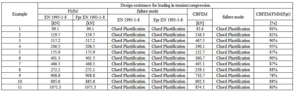
Studiul arată o bună concordanță pentru cazurile de încărcare aplicate. Rezultatele sunt rezumate într-un diagram care compară rezistențele de calcul ale CBFEM și FMM; a se vedea Fig. 7.2.3. Rezultatele arată că diferența dintre cele două metode de calcul este în toate cazurile mai mică de 10 %.

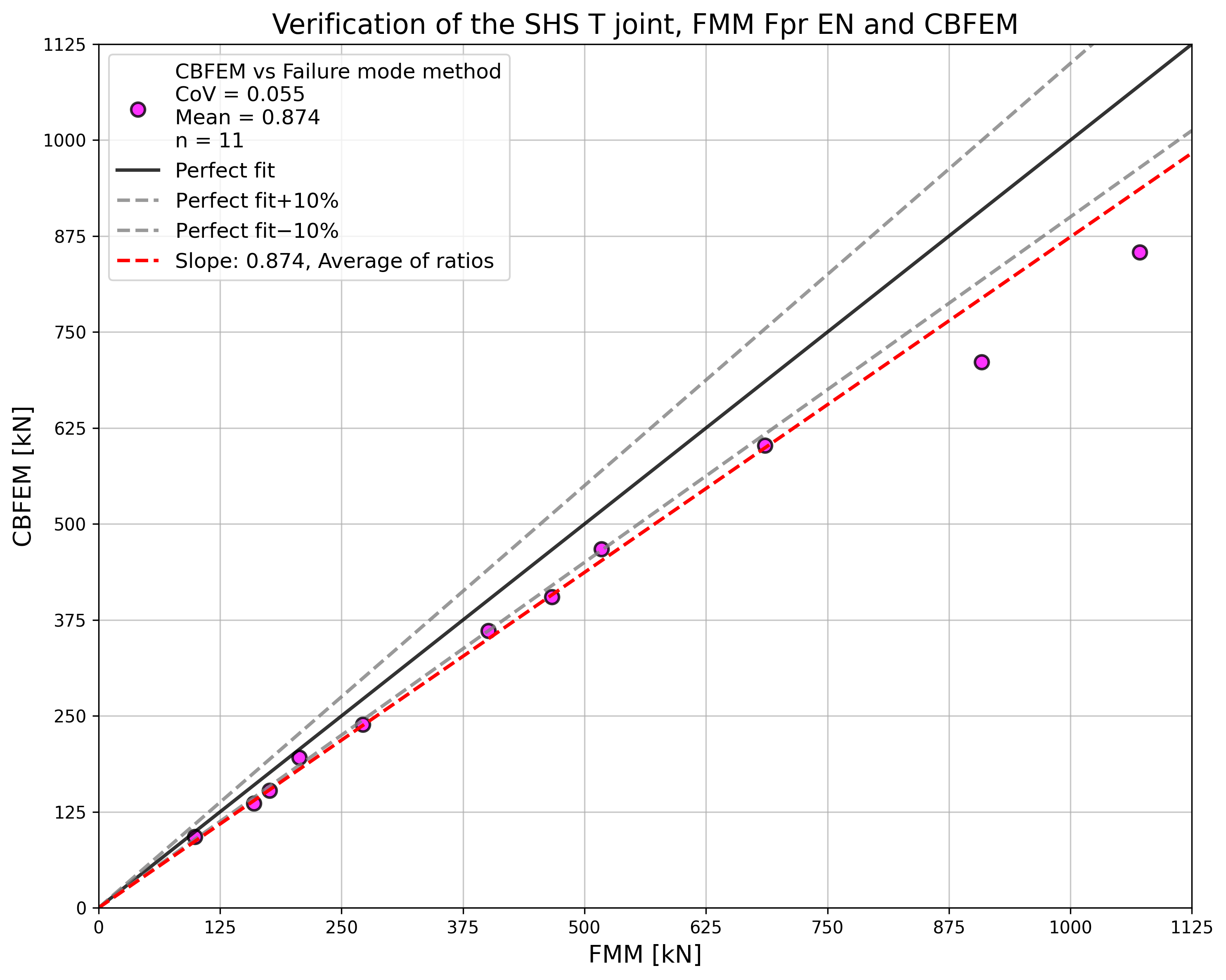
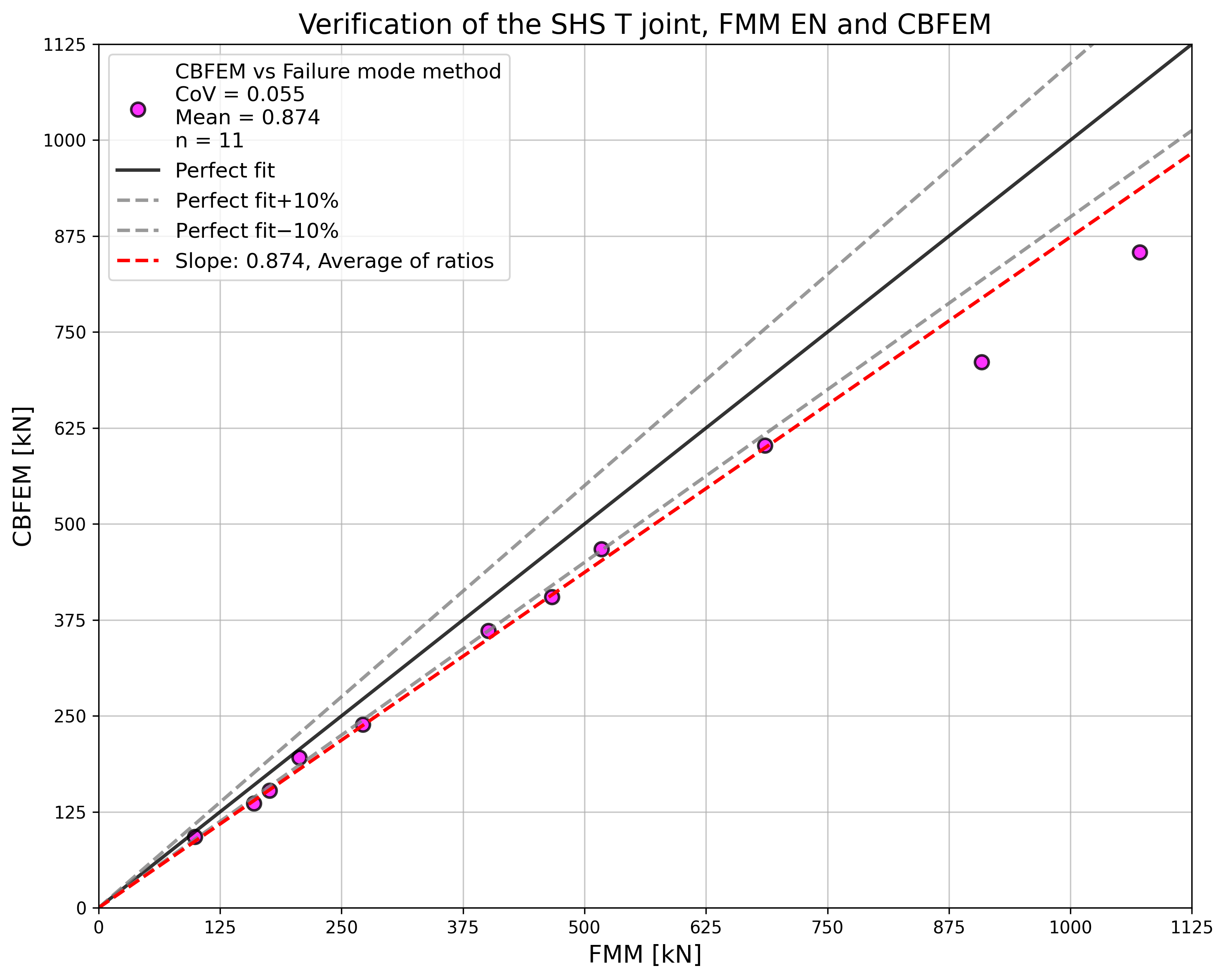
\[ \textsf{\textit{\footnotesize{Fig. 7.2.3 Verificarea rezistenței determinate prin CBFEM față de FMM pentru îmbinarea SHS T și Y uniplanară}}}\]

Exemplu de referință

Date de intrare

Talpă

• Oțel S355
• Secțiune SHS 200×200×6.3

Diagonală

• Oțel S355
• Secțiune SHS 90×90×8.0
• Unghi dintre diagonală și talpă 90°

Sudură

• Sudură cap la cap

Dimensiunea plasei

• 16 elemente pe cea mai mare inimă a elementului tubular dreptunghiular

Încărcare

• Prin forță aplicată diagonalei la compresiune/întindere

Rezultate

• Rezistența de calcul la compresiune/întindere este N_Rd = 92.6 kN
• Modul de cedare de calcul este cedarea feței tălpii

Îmbinare X-SHS uniplanară

O prezentare generală a exemplelor considerate este dată în Tab. 7.2.4. Cazurile selectate acoperă o gamă largă de raporturi geometrice ale îmbinărilor. Îmbinările selectate au cedat conform metodei bazate pe FMM prin cedarea feței tălpii sau cedarea diagonalei.

Tab. 7.2.4 Prezentare generală a exemplelor

Exemplu	Talpă	Diagonală	Unghiuri		Material
	Secțiune	Secțiune	θ	fy	fu	E
			[°]	[MPa]	[MPa]	[GPa]
1	SHS200/6.3	SHS140/12.5	90	355	490	210
2	SHS200/8.0	SHS70/8.0	90	355	490	210
3	SHS200/10.0	SHS120/12.5	90	355	490	210
4	SHS200/12.5	SHS90/8.0	90	355	490	210
5	SHS200/6.3	SHS90/8.0	60	355	490	210
6	SHS200/8.0	SHS80/8.0	60	355	490	210
7	SHS200/10.0	SHS150/6.3	60	355	490	210
8	SHS200/12.5	SHS140/12.5	60	355	490	210
9	SHS200/16.0	SHS120/12.5	60	355	490	210
10	SHS200/6.3	SHS100/8.0	30	355	490	210
11	SHS200/8.0	SHS150/16.0	30	355	490	210
12	SHS200/10.0	SHS100/10.0	30	355	490	210
13	SHS200/16.0	SHS90/8.0	30	355	490	210

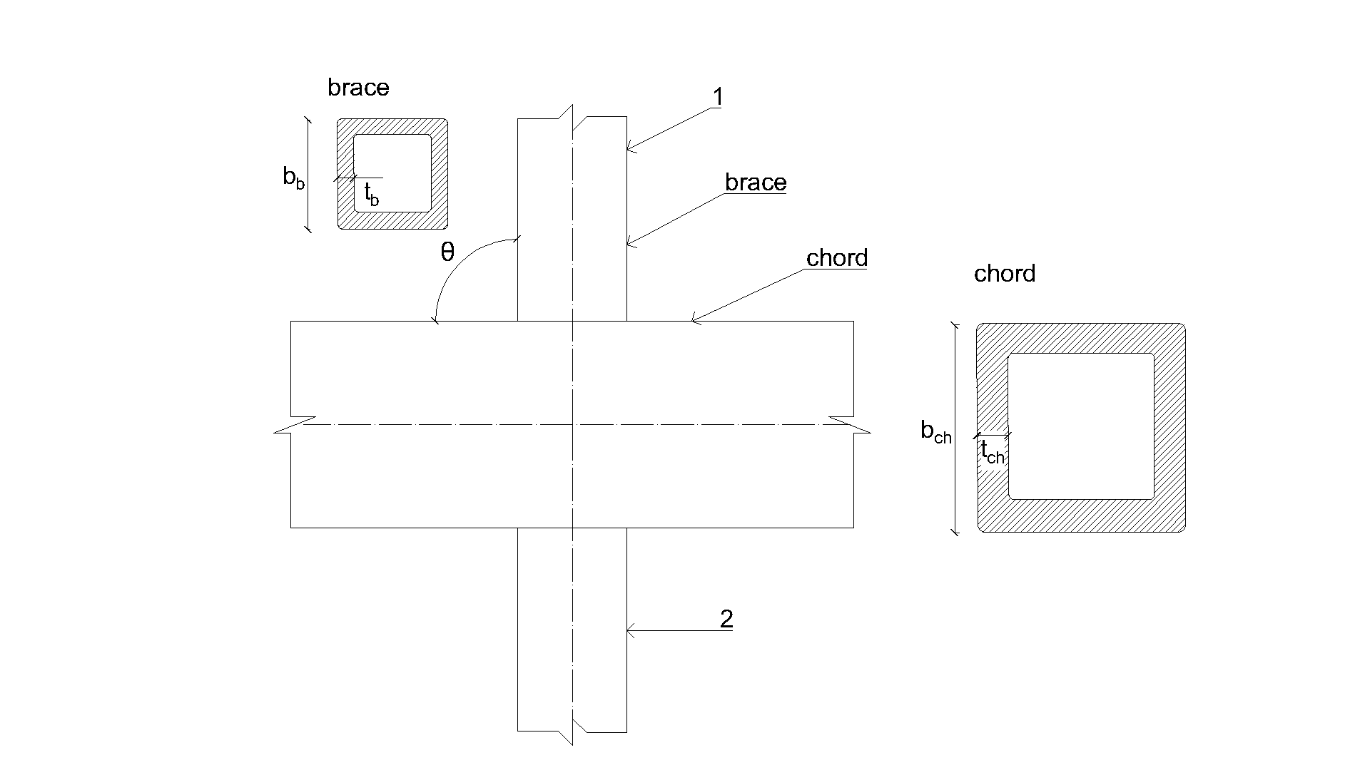
\[ \textsf{\textit{\footnotesize{Fig. 7.2.4 Dimensiunile îmbinării X}}}\]

Verificarea rezistenței

Rezultatele metodei bazate pe moduri de cedare (FMM) sunt comparate cu rezultatele CBFEM. Comparația este axată pe rezistență și modul de cedare de calcul; a se vedea Tab. 7.2.5.

Tab. 7.2.5 Compararea rezultatelor predicției rezistenței prin CBFEM și FMM

Studiul arată o bună concordanță pentru cazurile de încărcare aplicate. Rezultatele sunt rezumate într-un diagram care compară rezistențele de calcul ale CBFEM și FMM; a se vedea Fig. 7.2.4. Rezultatele arată că diferența dintre cele două metode de calcul este în toate cazurile mai mică de 13 %.

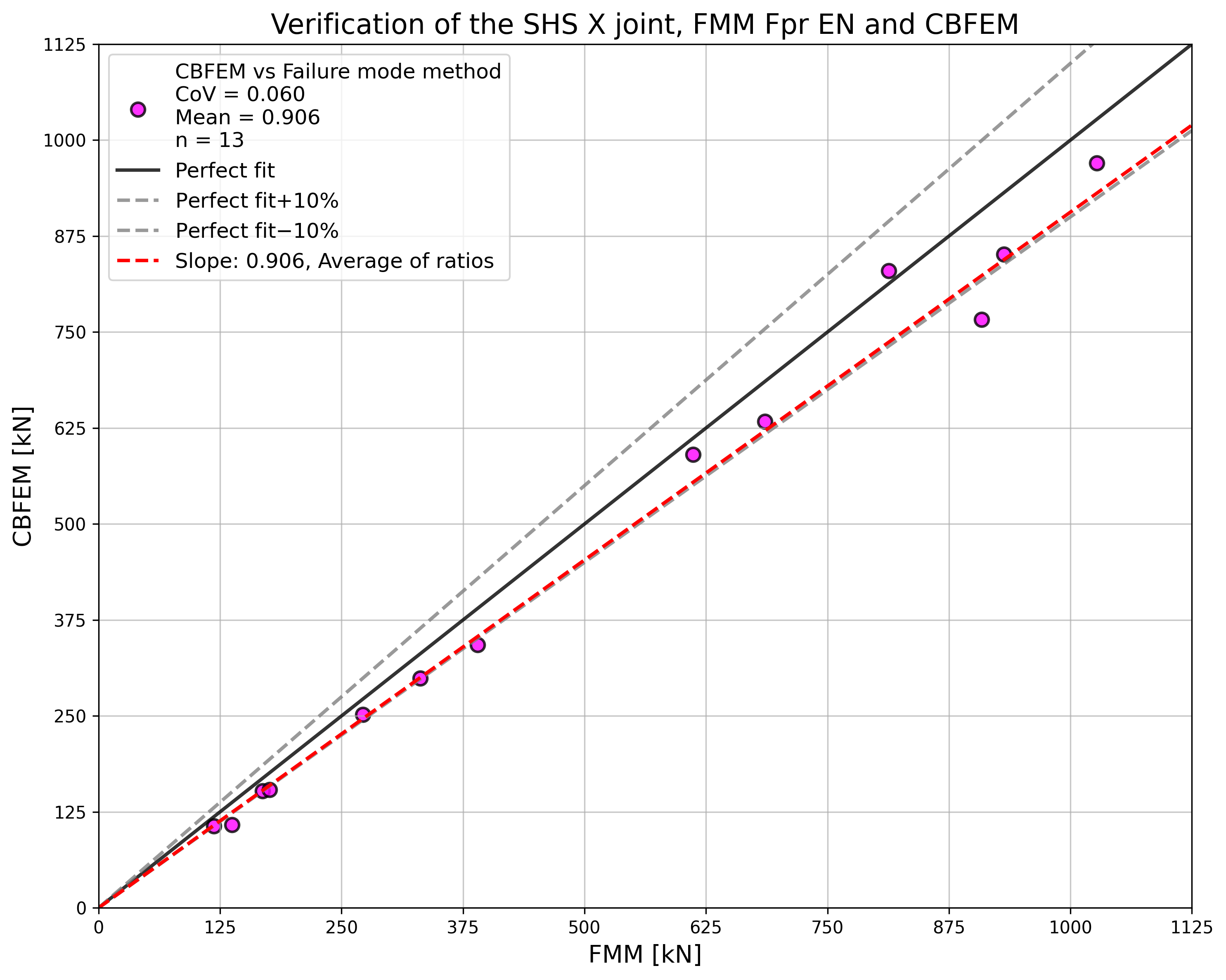
\[ \textsf{\textit{\footnotesize{Fig. 7.2.5 Verificarea rezistenței determinate prin CBFEM față de FMM pentru îmbinarea SHS X uniplanară}}}\]

Exemplu de referință

Date de intrare

Talpă

• Oțel S355
• Secțiune SHS 200×200×6,3

Diagonale

• Oțel S355
• Secțiuni SHS 140×140×12,5
• Unghi dintre diagonale și talpă 90°

Suduri

• Suduri cap la cap

Dimensiunea plasei

• 16 elemente pe cea mai mare inimă a elementului tubular dreptunghiular

Încărcare

• Prin forță aplicată diagonalei la compresiune/întindere

Rezultate

• Rezistența de calcul la compresiune/întindere este N_Rd = 152.4 kN
• Modul de cedare de calcul este cedarea feței tălpii

7.2.4 Îmbinare K-SHS uniplanară

O prezentare generală a exemplelor considerate este dată în Tab. 7.2.6. Cazurile selectate acoperă o gamă largă de raporturi geometrice ale îmbinărilor. Îmbinările selectate au cedat conform metodei bazate pe FMM prin cedarea feței tălpii sau cedarea diagonalei.

Tab. 7.2.6 Prezentare generală a exemplelor

Exemplu	Talpă	Diagonale	Unghiuri		Material
	Secțiune	Secțiuni	θ	fy	fu	E
			[°]	[MPa]	[MPa]	[GPa]
1	SHS180/10.0	SHS70/3.0	45	355	490	210
2	SHS180/10.0	SHS70/3.6	45	355	490	210
3	SHS200/8.0	SHS80/3.6	45	355	490	210
4	SHS200/8.0	SHS100/10.0	45	355	490	210
5	SHS200/200/10.0	SHS70/3.6	45	355	490	210
6	SHS200/200/10.0	SHS100/4.0	45	355	490	210
7	SHS200/200/12.5	SHS70/6.3	45	355	490	210
8	SHS200/200/12.5	SHS100/8.0	45	355	490	210

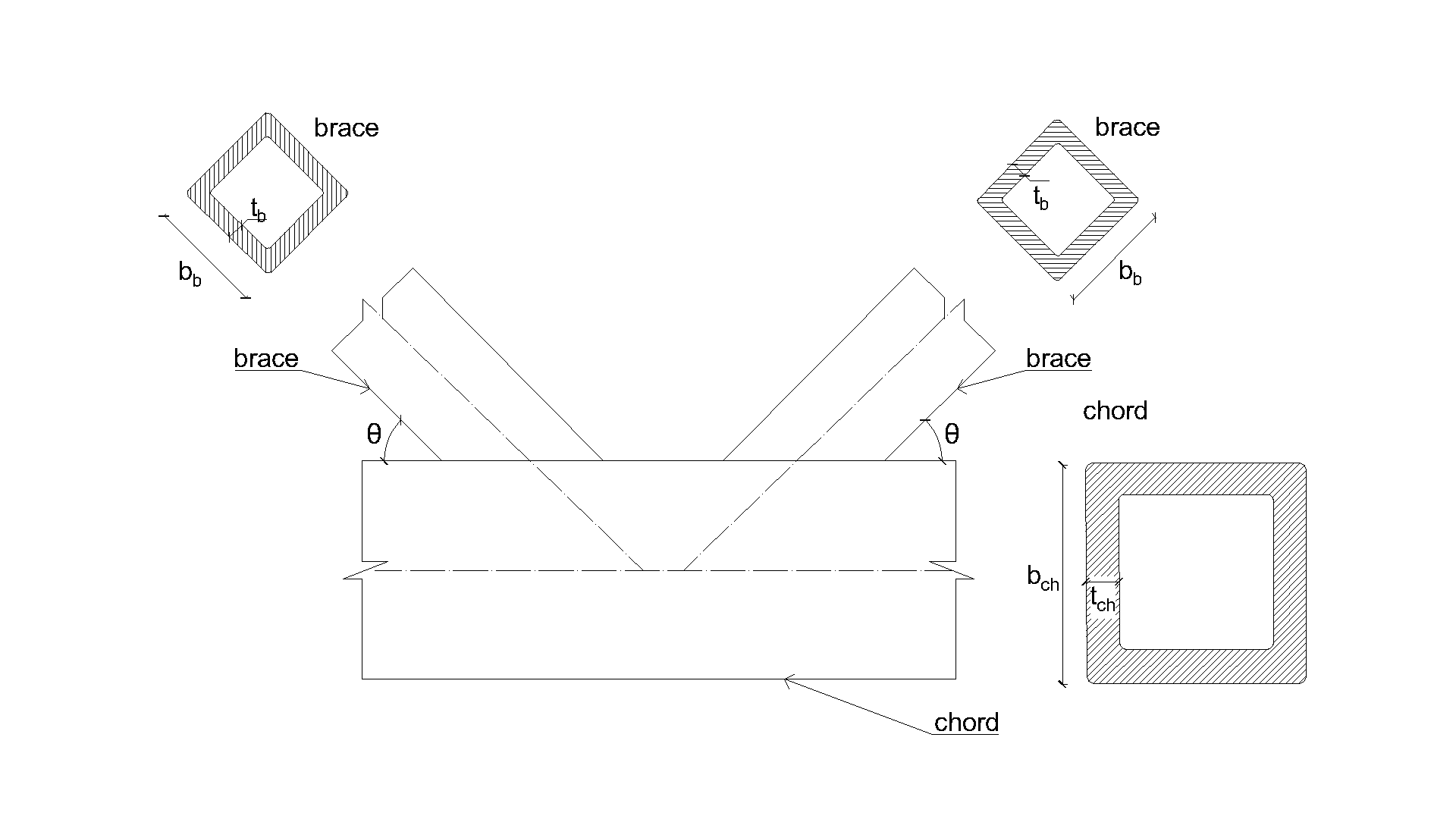
\[ \textsf{\textit{\footnotesize{Fig. 7.2.6 Dimensiunile îmbinării K}}}\]

Verificare

Rezultatele CBFEM sunt comparate cu rezultatele FMM. Comparația este axată pe rezistență și modul de cedare de calcul. Rezultatele sunt prezentate în Tab. 7.2.7.

Tab. 7.2.7 Compararea rezultatelor predicției rezistențelor prin CBFEM și FMM

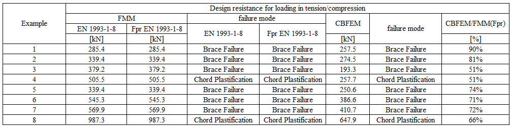
Studiul arată o bună concordanță pentru cazurile de încărcare aplicate. Rezultatele sunt rezumate într-un diagram care compară rezistențele de calcul ale CBFEM și FMM; a se vedea Fig. 7.2.5. Rezultatele arată că CBFEM este conservativ în toate cazurile față de FMM.

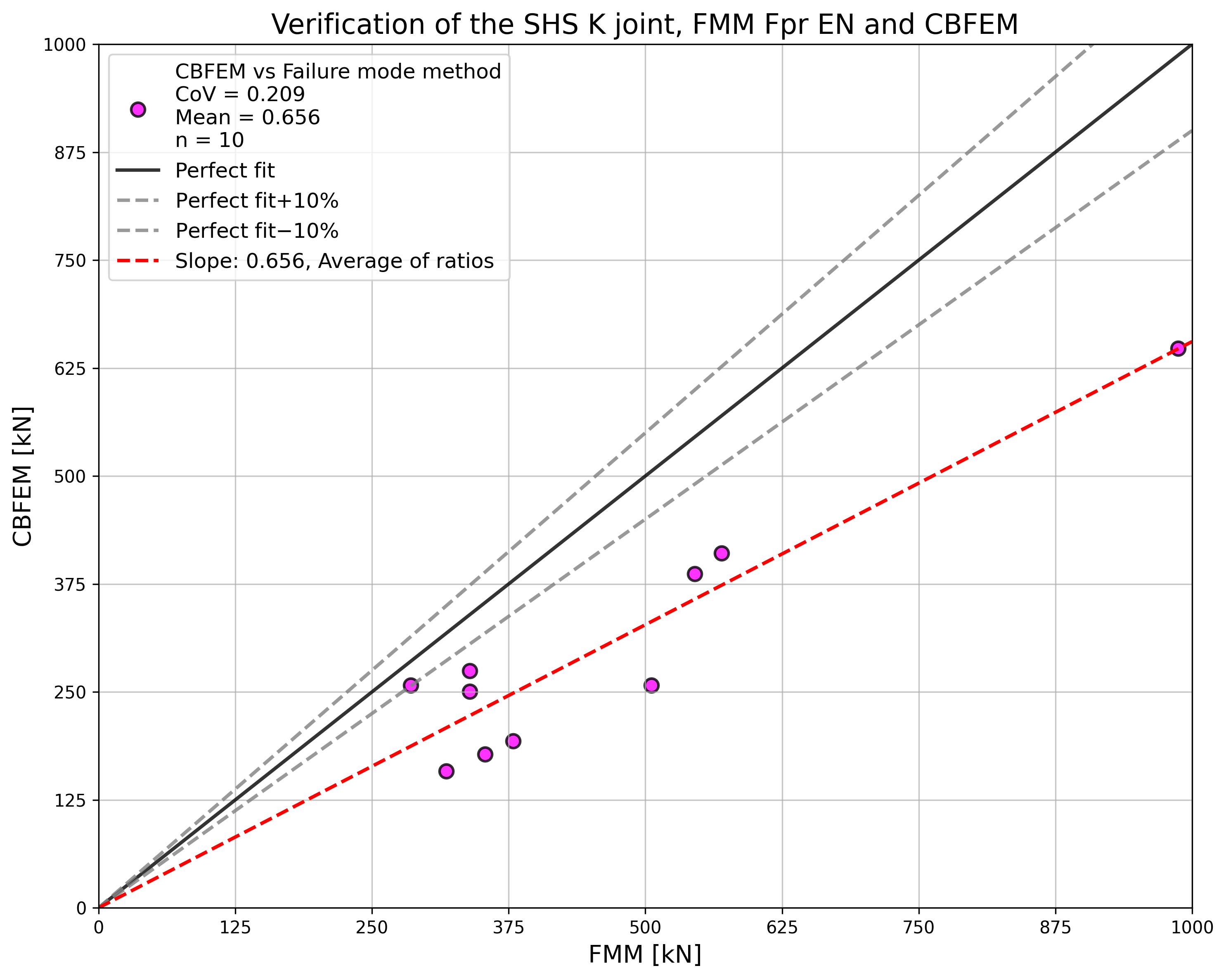
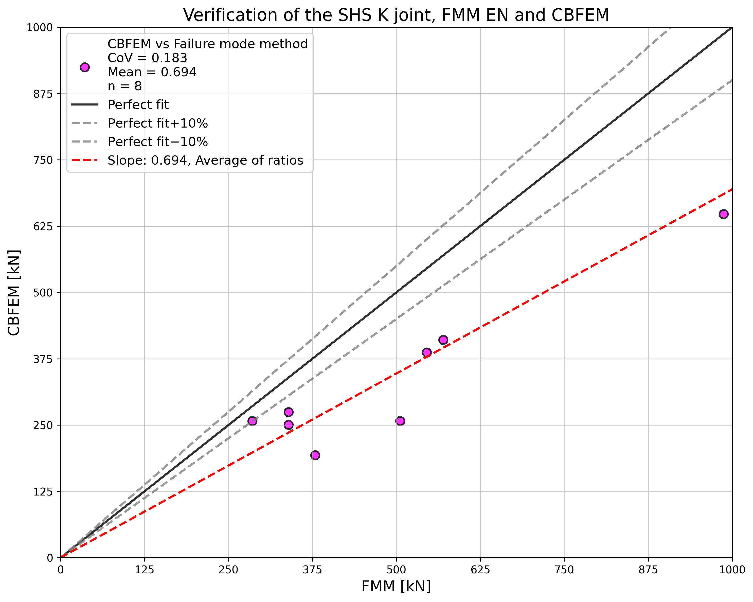
\[ \Fig. 7.2.7 Verificarea rezistenței determinate prin CBFEM față de FMM pentru îmbinarea SHS K uniplanară}}}\]

Exemplu de referință

Date de intrare

Talpă

• Oțel S355
• Secțiune SHS 180×180×10,0

Diagonale

• Oțel S355
• Secțiuni SHS 70×70×3,0
• Unghi dintre diagonale și talpă 45°

Suduri

• Suduri cap la cap

Dimensiunea plasei

• 16 elemente pe cea mai mare inimă a elementului tubular dreptunghiular

Încărcare

• Prin forță aplicată diagonalei la compresiune/întindere

Rezultate

• Rezistența de calcul la compresiune/întindere este N_Rd = 257.5 kN
• Modul de cedare de calcul este cedarea feței tălpii

Placă la secțiune tubulară circulară

Metoda modului de cedare

Îmbinările T uniplanare sudate placă-secțiune tubulară circulară, estimate prin CBFEM, sunt verificate față de FMM în acest capitol. În CBFEM, rezistența de calcul este limitată prin atingerea unei deformații de 5 % sau a unei forțe corespunzătoare unei deformații de 3 % d₀ a îmbinării, unde d₀ este diametrul tălpii. FMM se bazează pe limita de sarcină maximă sau pe limita de deformație de 3 % d₀; a se vedea Lu et al. (1994). Sudurile, proiectate conform EN 1993‑1‑8:2006, nu sunt componentele cele mai slabe ale îmbinării.

Plastificarea tălpii

Rezistența de calcul a feței tălpii CHS este determinată folosind metoda dată de modelul FMM din Cap. 9 al prEN 1993-1-8:2020 și din ISO/FDIS 14346; a se vedea Fig. 7.3.1. Rezistența de calcul a îmbinării sudate placă-CHS încărcate axial este:

Îmbinare T

Transversală

\[ N_{1,Rd} = 2.5 \cdot C_f f_{y0} t_0^2 (1+3 \beta^2) \gamma^{0.35} Q_f / \gamma_{M5} \]

Longitudinală

\[ N_{1,Rd} = 7.1 \cdot C_f f_{y0} t_0^2 (1+0.4 \eta) Q_f / \gamma_{M5} \]

Îmbinare X

Transversală

\[ N_{1,Rd} = 2.1 \cdotC_f f_{y0} t_0^2 (1+3 \beta^2) \gamma^{0.25} Q_f / \gamma_{M5} \]

Longitudinală

\[ N_{1,Rd} = 3.5 \cdotC_f f_{y0} t_0^2 (1+0.4 \eta^2) \gamma^{0.1} Q_f / \gamma_{M5} \]

unde:

• f_y,i – limita de curgere a elementului i (i = 0,1,2 sau 3)
• t_i – grosimea peretelui elementului CHS i (i = 0,1,2 sau 3)
• \(\beta\) – raportul dintre diametrul mediu sau lățimea elementelor diagonale și cel al tălpii
• \(\eta\) – raportul dintre înălțimea elementului diagonal și diametrul sau lățimea tălpii
• \(\gamma\) – raportul dintre lățimea sau diametrul tălpii și dublul grosimii peretelui său
• Q_f – factorul de tensiune al tălpii
• C_f – factorul de material
• \(\gamma_{M5}\) – factor parțial pentru rezistența îmbinărilor din grinzi cu zăbrele cu secțiuni tubulare
• N_i,Rd – rezistența de calcul a unei îmbinări exprimată în termenii forței axiale interioare din elementul i (i = 0,1,2 sau 3)

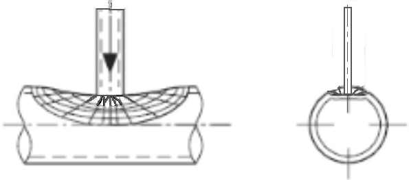
\[ \textsf{\textit{\footnotesize{Fig. 7.3.1 Modul de cedare examinat - plastificarea tălpii}}}\]

Domeniu de valabilitate

CBFEM a fost verificat pentru îmbinări tipice ale secțiunilor tubulare circulare sudate. Domeniul de valabilitate pentru aceste îmbinări este definit în Tabelul 7.8 din prEN 1993-1-8:2020; a se vedea Tab. 7.3.1. Același domeniu de valabilitate se aplică modelului CBFEM. În afara domeniului de valabilitate al FMM, trebuie pregătit un experiment pentru validare sau efectuată o verificare conform unui model de cercetare validat.

Tab. 7.3.1 Domeniu de valabilitate pentru metoda modurilor de cedare

General	\(0.2 \le \frac{d_i}{d_0} \le 1.0 \)	\( \theta_i \ge 30^{\circ} \)	\(-0.55 \le \frac{e}{d_0} \le 0.25 \)
	\(g \ge t_1+t_2 \)	\(f_{yi} \le f_{y0} \)	\( t_i \le t_0 \)

Talpă	Compresiune	Clasa 1 sau 2 și \(10 \le d_0 / t_0 \le 50 \) (dar pentru îmbinări X: \( d_0/t_0 \le 40 \))
	Întindere	\(10 \le d_0 / t_0 \le 50 \) (dar pentru îmbinări X: \( d_0/t_0 \le 40 \))
Placă transversală		\(0.25\le\beta=b_1/d_0\le1\)
Placă longitudinală		\(0.6\le\eta=h_1/d_0\le4 \)

Validare

În acest capitol, CBFEM este validat față de modelele FMM ale îmbinărilor T placă-CHS descrise în prEN 1993-1-8:2020. Modelele sunt comparate cu datele din testele mecanice din Tab. 7.3.2–7.3.3, cu rezistența bazată pe limita de deformație. Proprietățile de material și geometrice ale testelor numerice sunt descrise în (Voth A.P. și Packer A.J., 2010). Experimentele în afara domeniului de valabilitate sunt marcate în tabele cu asterisk * și indicate în grafic pentru a arăta calitatea condițiilor la limită.

Tab. 7.3.2 Proprietăți geometrice, proprietăți de material și rezistențele îmbinărilor din experimente și modele FMM pentru îmbinarea T transversală

ID	Referință	d0 [mm]	t0 [mm]	h1 [mm]	h1/d0 [-]	d0/t0 [-]	fy0 [MPa]
TPT 1	Washio et al. (1970)	165,2	5,2	115,6	0,7	31,8	308,0
TPT 2	Washio et al. (1970)	165,2	5,2	148,7	0,9	31,8	308,0
TPT 3	Washio et al. (1970)	139,8	3,5	125,8	0,9	39,9	343,0
TPT 4	Voth et al. (2012)	219,2	4,5	100,3	0,5	48,8	388,8

ID	Nu,exp [kN]	Tip ramură	Nu,exp/(t02·fy0)	N1,prEN/(t02·fy0)	Nu,exp/N1,prEN
TPT 1	169,4	Compresiune	20,34	16,25	1,25
TPT 2	250,5	Compresiune	30,08	22,58	1,33
TPT 3	184,8	Compresiune	43,98	24,45	1,80
TPT 4	282,5	Întindere	36,04	12,45	2,89

Tab. 7.3.3 Proprietăți geometrice, proprietăți de material și rezistențele îmbinărilor din experimente și modele FMM pentru îmbinarea T longitudinală

ID	Referință	d0 [mm]	t0 [mm]	h1 [mm]	h1/d0 [-]	d0/t0 [-]	fy0 [MPa]
TPL 1	Washio et al. (1970)	165,2	5,2	165,2	1,0	31,8	308,0
TPL 2	Washio et al. (1970)	165,2	5,2	330,4	2,0	31,8	308,0
*TPL 3	Voth et al. (2012)	219,2	4,5	99,9	0,5	48,8	388,8

ID	Nu,exp [kN]	Tip ramură	Nu,exp/(t02·fy0)	N1,prEN/(t02·fy0)	Nu,exp/N1,prEN
TPL 1	107,6	Compresiune	12,92	10,36	1,25
TPL 2	127,4	Compresiune	15,30	13,32	1,15
*TPL 3	160,6	Întindere	20,49	8,75	2,34

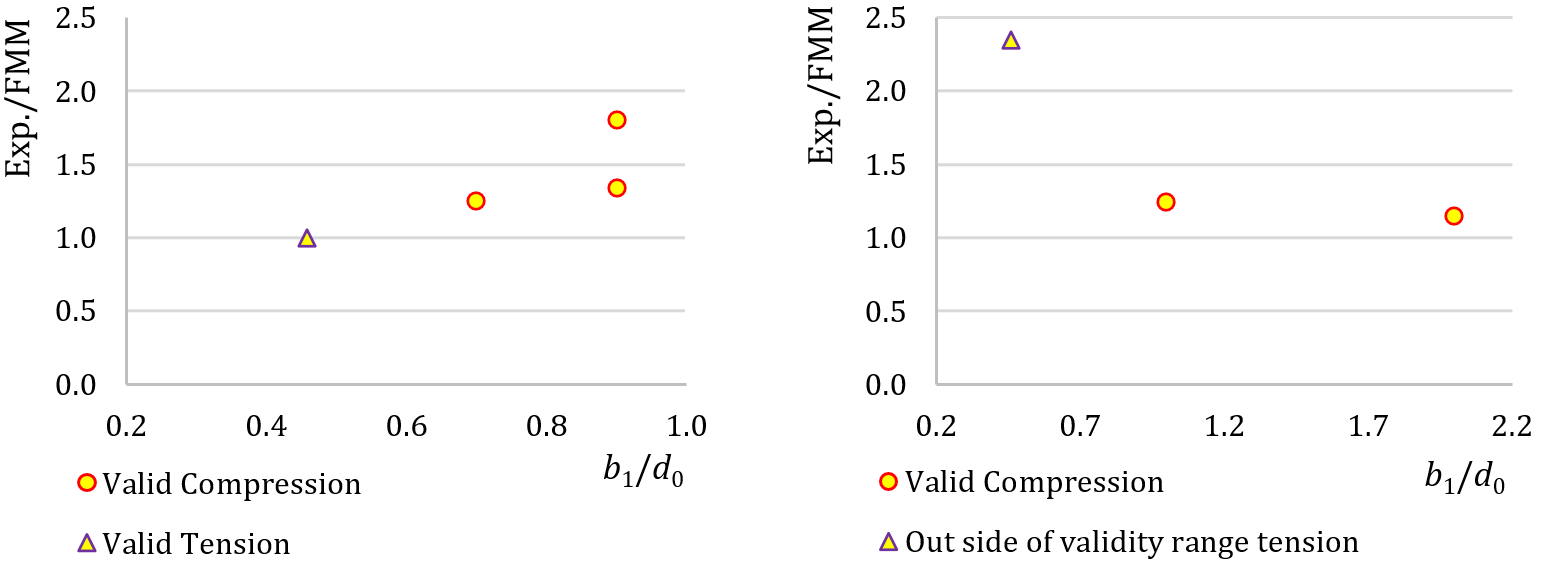
\[ \textsf{\textit{\footnotesize{ Fig. 7.3.2 Validarea FMM față de experimentele mecanice pentru îmbinări T transversale placă-CHS (stânga) și pentru îmbinări T longitudinale placă-CHS (dreapta)}}}\]

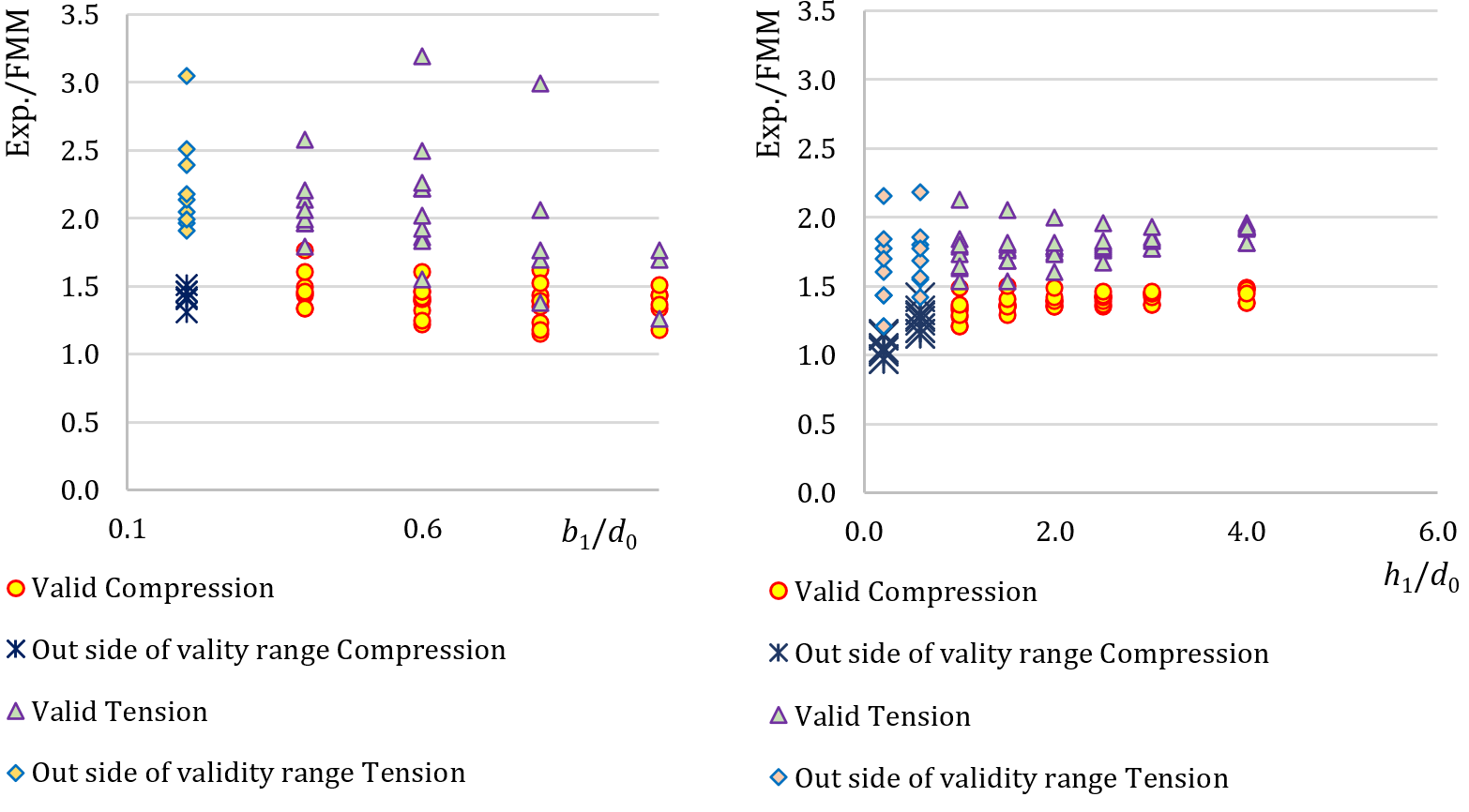
\[ \textsf{\textit{\footnotesize{Fig. 7.3.3 Validarea FMM față de experimentele mecanice pentru îmbinări T transversale placă-CHS (stânga) și îmbinări T longitudinale placă-CHS (dreapta)}}}\]

Validarea prezentată în Fig. 7.3.2 și 7.3.3 demonstrează că diferențele față de experimente sunt de cel puțin 15 % în general, pe partea sigură. Experimentele în afara domeniului de valabilitate sunt incluse și marcate. Rezultatele indică calitatea bună a condițiilor la limită alese.

Îmbinare T uniplanară placă

O prezentare generală a exemplelor considerate în studiu este dată în Tab. 7.3.4. Cazurile selectate acoperă o gamă largă de rapoarte geometrice ale îmbinărilor. Geometria îmbinărilor cu dimensiuni este prezentată în Fig. 7.3.4. Grosimea plăcii este de 15 mm în toate cazurile acoperite în acest studiu.

Tab. 7.3.4 Prezentare generală a exemplelor

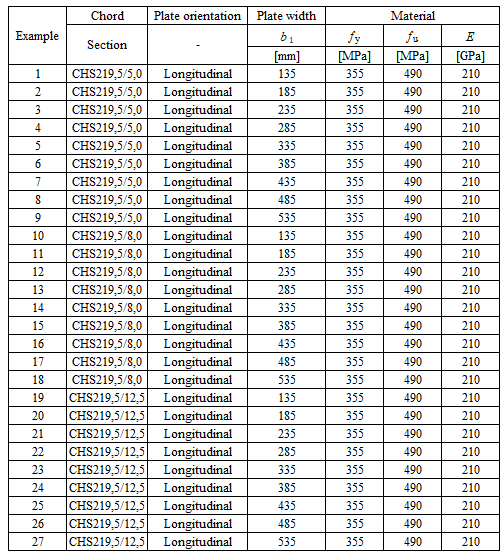
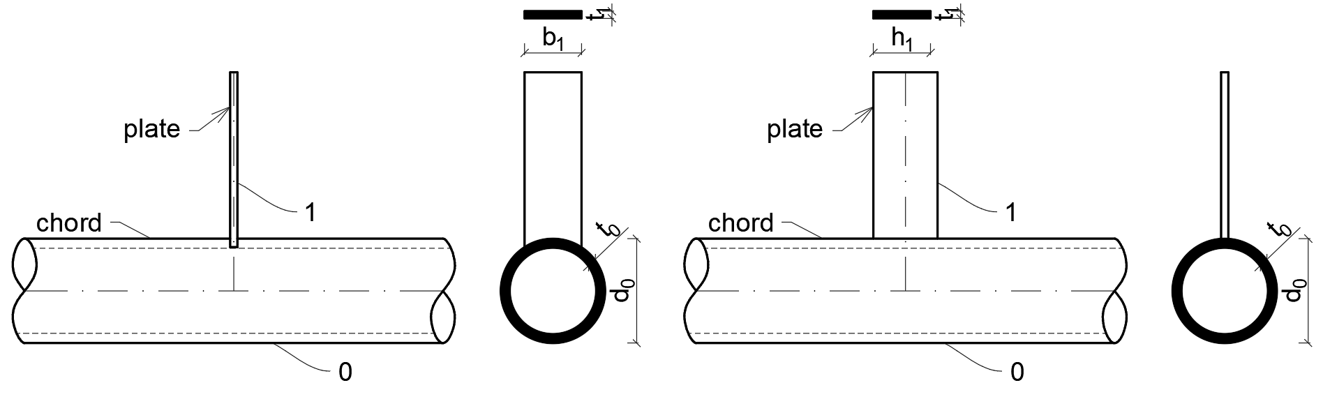
\[ \textsf{\textit{\footnotesize{Fig. 7.3.4 Dimensiunile îmbinării T placă-CHS, transversală (stânga) și longitudinală (dreapta)}}}\]

Verificare

Rezultatele rezistenței și ale modului de cedare de calcul din FMM sunt comparate cu rezultatele CBFEM în Tab. 7.3.5 și în Fig. 7.3.5.

Tab. 7.3.5 Verificarea predicției rezistențelor prin CBFEM față de FMM a) orientare transversală  b) orientare longitudinală

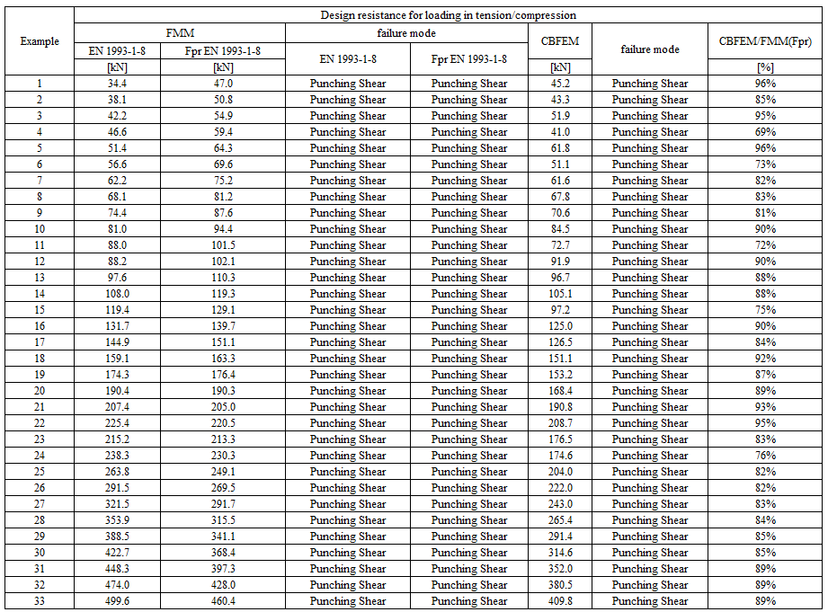
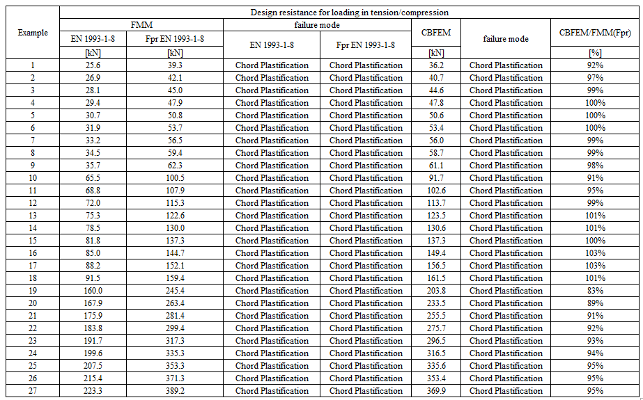
Studiul arată o concordanță bună pentru cazurile de încărcare aplicate. Rezultatele sunt rezumate în diagrame care compară rezistențele de calcul ale CBFEM și FMM; a se vedea Fig. 7.3.5. Rezultatele arată că diferența dintre cele două metode de calcul este în toate cazurile mai mică de 7 %.

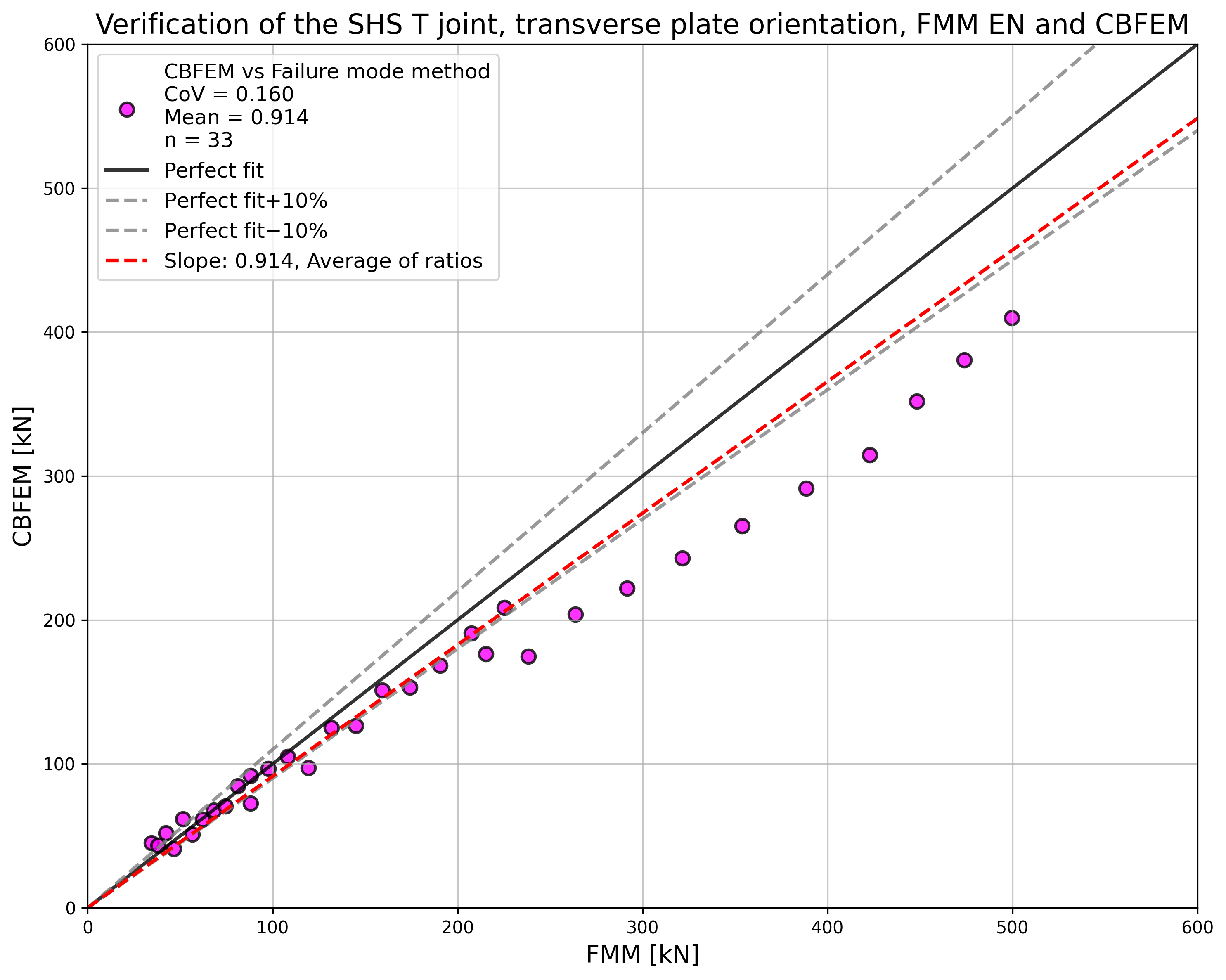
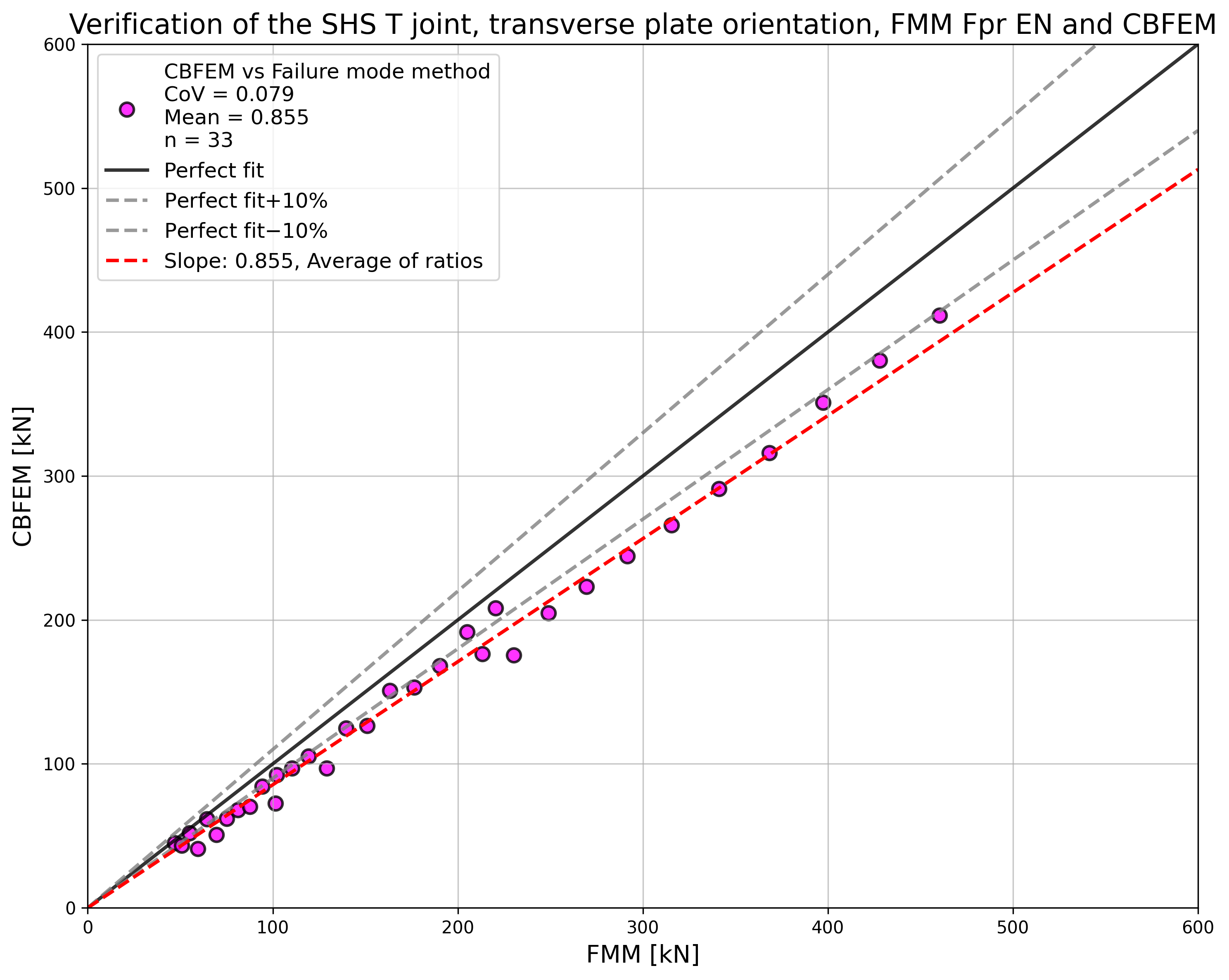
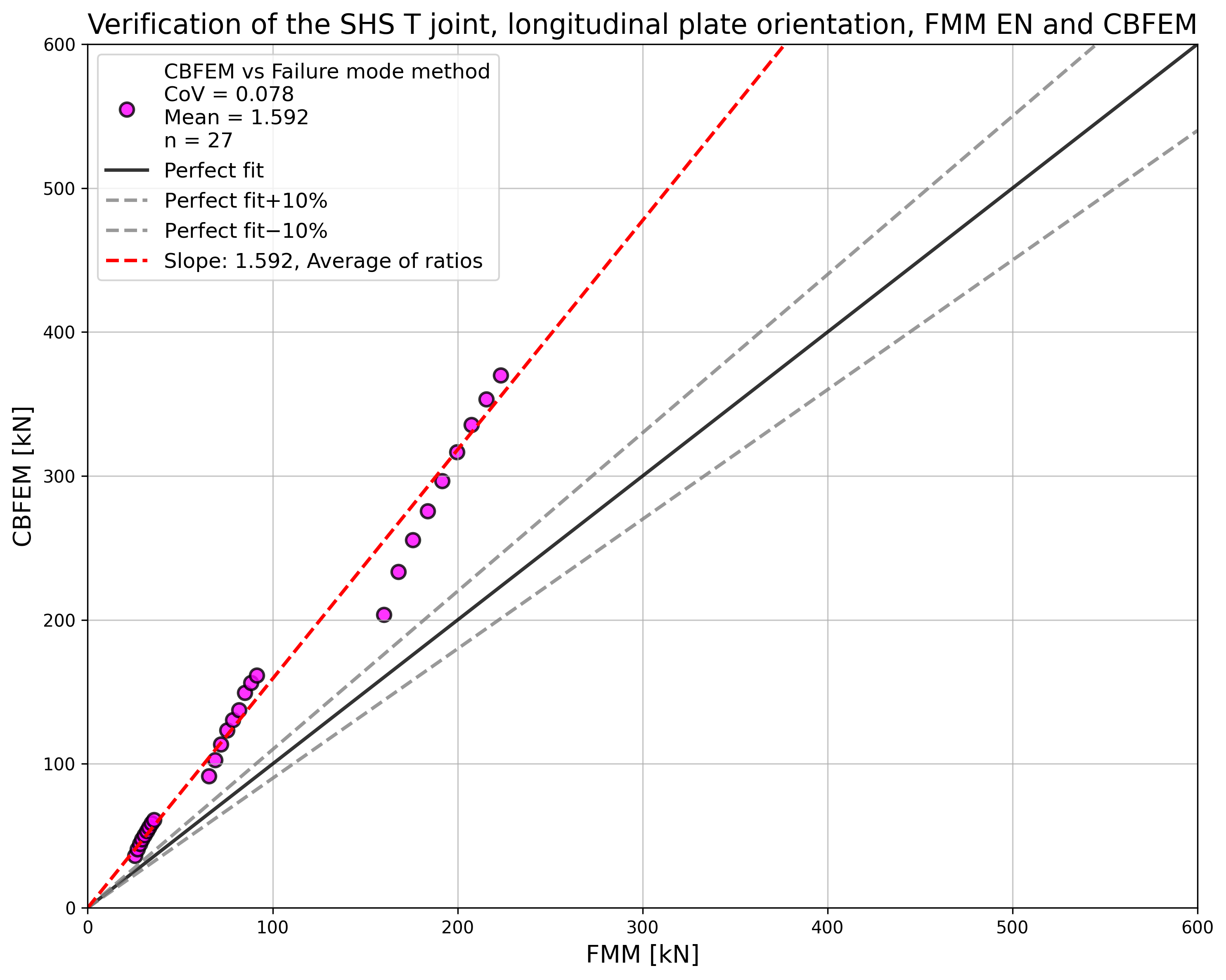
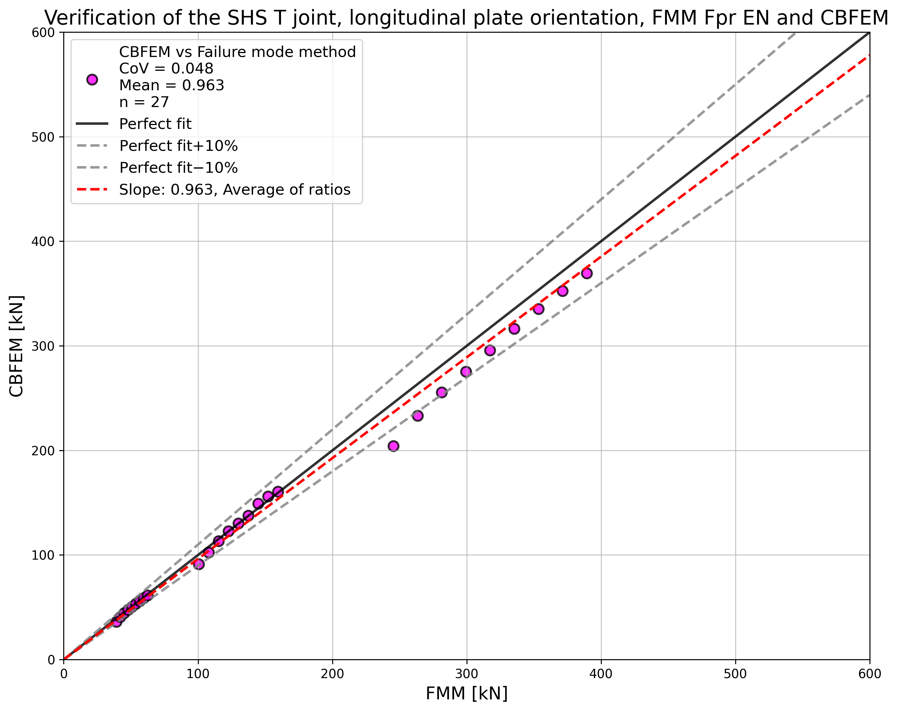
\[ \textsf{\textit{\footnotesize{Fig. 7.3.5 Verificarea CBFEM față de FMM pentru îmbinarea T uniplanară placă-CHS}}}\]

Exemplu de referință

Date de intrare

Talpă

• Oțel S355
• Secțiune CHS219.1/5,0

Ramură

• Oțel S355
• Placă 95/15 mm
• Unghi între elementul ramură și talpă 90° (transversal)

Sudură

• Sudură cap la cap în jurul ramurii

Încărcare

• Prin forță pe ramură la compresiune

Dimensiunea plasei

• 64 elemente de-a lungul suprafeței elementului tubular circular

Date de ieșire

• Rezistența de calcul la compresiune este N_Rd = 45,2 kN
• Modul de cedare de calcul este forfecarea prin poansonare

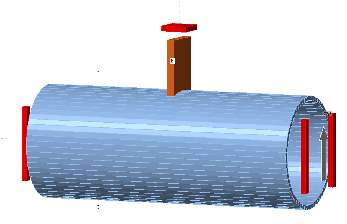
\[ \textsf{\textit{\footnotesize{Fig. 7.3.6 Condiții la limită pentru îmbinarea T uniplanară placă-CHS}}}\]

Îmbinare T uniplanară între un element diagonal RHS și un talpă H/I

Descriere

Se studiază o îmbinare T uniplanară a unui element diagonal cu secțiune tubulară dreptunghiulară (RHS) cu o talpă cu secțiune deschisă, situată într-un grătar cu zăbrele. Elementul diagonal RHS este sudat direct pe talpa H sau I, secțiuni deschise, fără utilizarea plăcilor de ranforsare. Predicția prin metoda elementelor finite bazată pe componente (CBFEM) este verificată cu metoda modurilor de cedare (FM) implementată în EN 1993-1-8:2005.

Model analitic

În îmbinarea T uniplanară a secțiunilor tubulare dreptunghiulare sudate cu secțiunile deschise apar trei moduri de cedare: curgerea locală a elementului diagonal, numită cedarea elementului diagonal, cedarea inimii tălpii și forfecarea tălpii. Toate aceste moduri de cedare sunt examinate în acest studiu; a se vedea Fig. 7.4.1. Sudurile sunt proiectate astfel încât să nu fie componenta cea mai slabă a unui nod, conform EN 1993-1-8:2005. Elementele grătarelor cu zăbrele sunt solicitate de forțe normale și momente încovoietoare. Punctul de acțiune al forțelor interioare ale îmbinării T este descris după cum urmează:

Talpă H/I solicitată axial

Forțele normale din talpa din dreapta și din stânga unei îmbinări T acționează în direcția axei longitudinale a tălpii.

Talpă H/I solicitată la difracție

Momentele încovoietoare din dreapta și din stânga unei îmbinări T în planul îmbinării T sunt considerate în talpă, iar aceste momente încovoietoare se rotesc în jurul uneia dintre axele din planul secțiunii transversale a tălpii pentru rotația în planul îmbinării T.

Element diagonal RHS solicitat axial

Forța normală din elementul diagonal al unei îmbinări T acționează în direcția axei longitudinale a elementului diagonal.

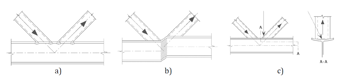
\[ \textsf{\textit{\footnotesize{Fig. 7.4.1 Moduri principale de cedare a) cedarea inimii tălpii, b) forfecarea tălpii (în cazul unui rost), c) cedarea elementului diagonal}}}\]

Rezistența inimii tălpii este determinată folosind metoda prezentată în secțiunea 7.6 din EN 1993-1-8:2005, descrisă în (Wardenier et al., 2010). Tensiunile din elementul diagonal sunt transferate prin talpa cornier a tălpii către o arie efectivă a inimii tălpii. Această arie este situată în inima tălpii în punctul în care pereții elementului diagonal intersectează inima tălpii. Rezistența axială de calcul a nodului este minimul rezistențelor de calcul:

Cedarea inimii tălpii

\[N_{\mathrm{i,Rd}} = \frac{f_{\mathrm{y0}} \cdot t_{\mathrm{w}} \cdot b_{\mathrm{w}}}{\sin(\theta_{\mathrm{i}}) \cdot \gamma_{\mathrm{M5}}}\]

Forfecarea tălpii

\[N_{i,\mathrm{Rd}}=\frac{f_\mathrm{y0}\,A_\mathrm{v}}{\sqrt{3}\,\sin\theta_\mathrm{i}\cdot \gamma_{\mathrm{M5}}}\]

Cedarea elementului diagonal

\[N_{i,\mathrm{Rd}}=2\,f_\mathrm{y1}\,t_\mathrm{1}\,p_{\mathrm{eff}}/\gamma_{\mathrm{M5}}\]

unde

\[p_{\mathrm{eff}}=t_\mathrm{w}+2r+7\,t_\mathrm{f}\,\frac{f_\mathrm{y0}}{f_\mathrm{y1}}\]

și \(A_\mathrm{v}\) este aria efectivă la forfecare.

Rezistența la încovoiere de calcul a nodului este minimul rezistențelor de calcul:

Cedarea inimii tălpii

\[M_{\mathrm{ip,Rd}} = \frac{0.5 \, f_{\mathrm{y0}} \, t_{\mathrm{w}} \, b_{\mathrm{w}} \, h_1}{\gamma_{\mathrm{M5}}}\]

Cedarea elementului diagonal

\[M_{\mathrm{ip,Rd}}=f_\mathrm{y1}\,t_\mathrm{1}\,b_{\mathrm{eff}}\,(h_\mathrm{1}-t_\mathrm{1})/\gamma_{\mathrm{M5}}\]

unde

\[b_{\mathrm{w}} = \frac{h_1}{\sin \theta_{\mathrm{i}}} + 5 \cdot t_{\mathrm{f,0}} + r \;\leq\; 2 \, t_{\mathrm{i}} + 10 \cdot (t_{\mathrm{f,0}} + r)\]

\[b_{\mathrm{eff}}=t_\mathrm{w}+2r+7\,t_\mathrm{f}\,\frac{f_\mathrm{y0}}{f_\mathrm{y1}}\]

O prezentare generală a exemplelor considerate solicitate de forță axială este descrisă în Tab. 7.4.1. O prezentare generală a exemplelor considerate solicitate de moment încovoietor este descrisă în Tab. 7.4.2. Geometria unui nod cu dimensiuni este prezentată în Fig. 7.4.2.

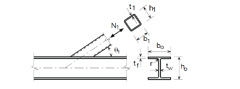
\[ \textsf{\textit{\footnotesize{Fig. 7.4.2 Geometria nodului cu dimensiuni}}}\]

Tab. 7.4.1 Exemple de noduri solicitate de forță axială 

Tab. 7.4.2 Exemple de noduri solicitate de moment în plan

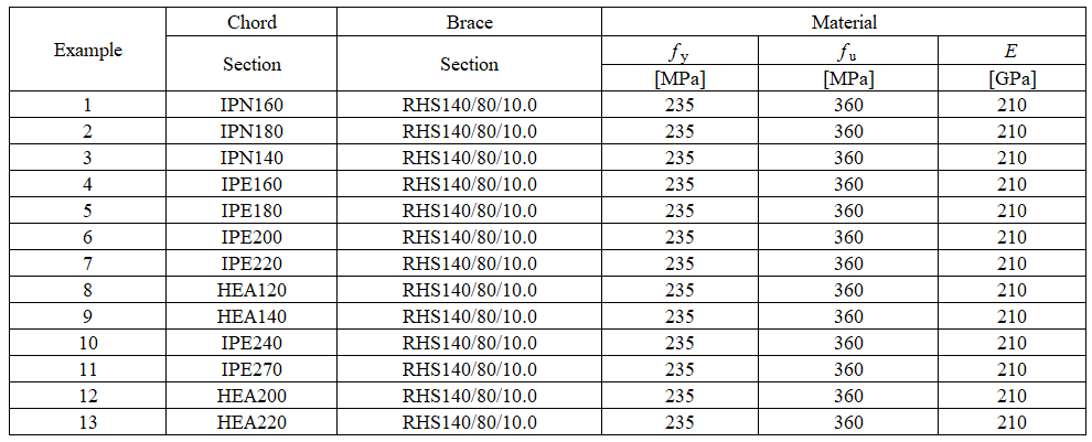
Verificarea rezistenței

Studiul s-a concentrat pe compararea modurilor de cedare și predicția rezistenței de calcul. Rezultatele sunt prezentate în Tab. 7.4.3 și 7.4.4.

Tab. 7.4.3 Comparație între CBFEM și FM pentru forța axială în elementul diagonal

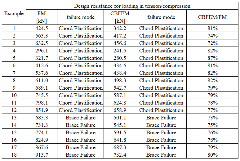
Tab. 7.4.4 Comparație între CBFEM și FM pentru momentul în plan în elementul diagonal

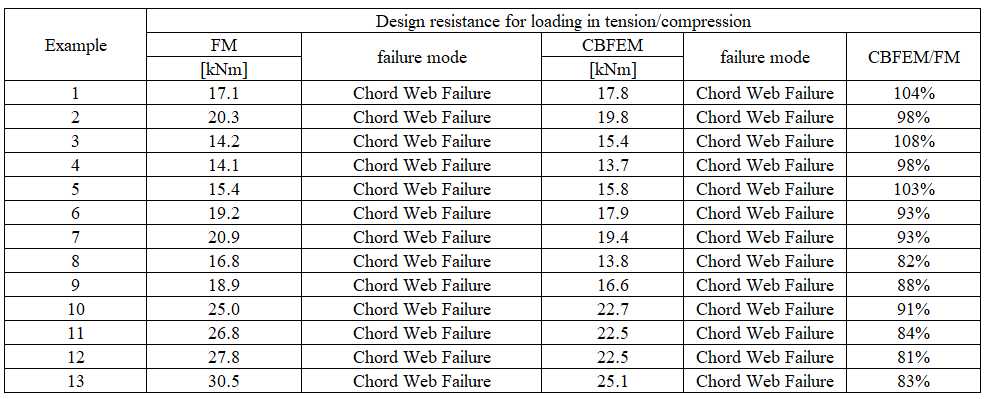
Studiul de sensibilitate arată o bună concordanță pentru toate cazurile de încărcare aplicate. În metoda CBFEM, rotunjirea peretelui secțiunii transversale deschise este simplificată, ceea ce conduce la o estimare conservatoare a tensiunii în elementul diagonal conectat și la ipoteza capacității portante până la 15%. Pentru a ilustra acuratețea modelului CBFEM, rezultatele studiilor parametrice sunt rezumate într-o diagramă care compară rezistențele de calcul prin CBFEM și FM; a se vedea Fig. 7.4.3.

\[ \textsf{\textit{\footnotesize{ Fig. 7.4.3 Verificarea CBFEM față de FM pentru forța axială și momentul încovoietor în elementul diagonal}}}\]

Domeniu de valabilitate

Domeniul de valabilitate pentru care CBFEM este verificat pentru îmbinările T între secțiuni tubulare dreptunghiulare și secțiuni deschise este definit în Tabelul 7.20 din EN 1993-1-8:2005, a se vedea Tab. 7.4.5. În cazul aplicării modelului CBFEM în afara domeniului de valabilitate al FM, trebuie pregătită validarea față de experimente sau verificarea față de un model de cercetare validat pentru a confirma calitatea predicției.

Tab. 7.4.5 Domeniu de valabilitate al îmbinărilor T

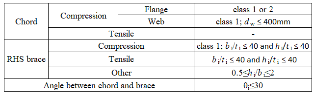
Exemplu de referință

Date de intrare

Talpă
• Oțel S235
• IPN280

Element diagonal
• Oțel S235
• RHS 140×80×10

Dimensiunea plasei
• 16 elemente pe cea mai mare inimă a elementului tubular dreptunghiular

Rezultate

• Rezistența de calcul la compresiune/întindere F_c,Rd = 457 kN (Se menționează că rezistența a fost calculată folosind funcția „Stop la deformația limită". În consecință, rezistența CBFEM reală poate fi marginal mai mare.)

• Modul de cedare este plastificarea tălpii

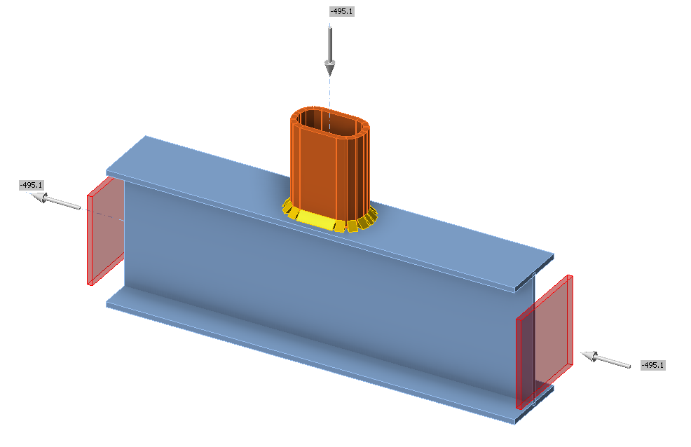
\[ \textsf{\textit{\footnotesize{Fig. 7.4.4 Exemplu de referință pentru talpa IPE270 și elementul diagonal RHS 140×80×10}}}\]

Baza stâlpului

Placă de bază – Element stâlp cu secțiune deschisă la compresiune

Descriere

În acest capitol, Metoda Elementelor Finite bazată pe componente (CBFEM) a plăcii de bază sub un stâlp metalic cu secțiune deschisă încărcat la compresiune pură este verificată prin metoda componentelor (MC). Studiul este elaborat pentru secțiunea transversală a stâlpului, dimensiunile plăcii de bază, clasa betonului și dimensiunile blocului de beton.

Metoda componentelor

Sunt luate în considerare trei componente: talpa și inima stâlpului la compresiune, betonul la compresiune inclusiv stratul de nivelare, sudurile. Componenta talpa și inima stâlpului la compresiune este descrisă în EN 1993-1-8:2005 Cl. 6.2.6.7. Betonul la compresiune inclusiv stratul de nivelare este modelat conform EN 1993-1-8:2005 Cl. 6.2.6.9 și EN 1992-1-1:2005 Cl. 6.7. Două iterații ale ariei efective sunt utilizate pentru determinarea rezistenței.

Sudura este proiectată în jurul secțiunii transversale a stâlpului; a se vedea EN 1993-1-8:2005 Cl. 4.5.3.2(6). Grosimea sudurii pe tălpi este aleasă egală cu grosimea sudurii pe inimă. Forța tăietoare este transferată numai prin sudurile de pe inimă, iar distribuția plastică a tensiunilor este considerată.

Placă de bază sub HEB 240

Acest studiu este axat pe componenta beton la compresiune inclusiv stratul de nivelare. Un exemplu de calcul este prezentat mai jos pentru blocul de beton cu dimensiunile a' = 1000 mm, b' = 1500 mm, h = 800 mm din beton clasa C20/25 cu placă de bază cu dimensiunile a = 330 mm, b = 440 mm, t = 20 mm din oțel S235; a se vedea Fig. 8.1.2.

 Rezistența îmbinării betonului este calculată sub aria efectivă la compresiune în jurul secțiunii transversale; a se vedea Fig. 8.1.1, iterând în două etape.

Pentru etapa 1^st este:

\[ f_{jd} = \frac{\beta_j k_j f_{ck}}{\gamma_c} = \frac{0.67 \cdot 2.908 \cdot 20}{1.5} = 26 \textrm{ MPa} \]

\[ c = t \sqrt{\frac{f_y}{3f_{jd} \gamma_{M0}}} = 20 \sqrt{\frac{235}{3 \cdot 26 \cdot 1.0}} = 35 \textrm{ mm} \]

 \[ l_{eff} = b+2c = 240+2\cdot35=310 \textrm{ mm} \]

 \[ b_{eff} = t_f+2c = 17+2\cdot35=87\textrm{ mm} \]

și pentru etapa 2^nd este:

\[ f_{jd} = \frac{\beta_j k_j f_{ck}}{\gamma_c} = \frac{0.67 \cdot 3 \cdot 20}{1.5} = 27 \textrm{ MPa} \]

\[ c = t \sqrt{\frac{f_y}{3f_{jd} \gamma_{M0}}} = 20 \sqrt{\frac{235}{3 \cdot 27 \cdot 1.0}} = 34 \textrm{ mm} \]

 \[ l_{eff} = b+2c = 240+2\cdot35=308 \textrm{ mm} \]

 \[ b_{eff} = t_f+2c = 17+2\cdot35=85\textrm{ mm} \]

\[A_{eff} = 63463 \textrm{ mm}^2\]

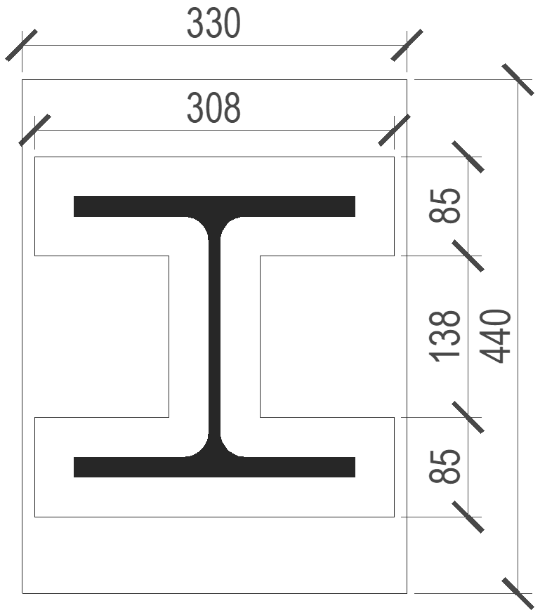
Fig. 8.1.1 Aria efectivă sub placa de bază

Rezistența la forță normală a plăcii de bază prin MC este

\[N_{Rd} = A_{eff} \cdot f_{jd} = 63436 \cdot 27 = 1701 \textrm{ kN} \]

Tensiunile calculate prin CBFEM sunt prezentate în Fig. 8.1.2. Rezistența la forță normală de compresiune a plăcii de bază prin CBFEM este 1683 kN.

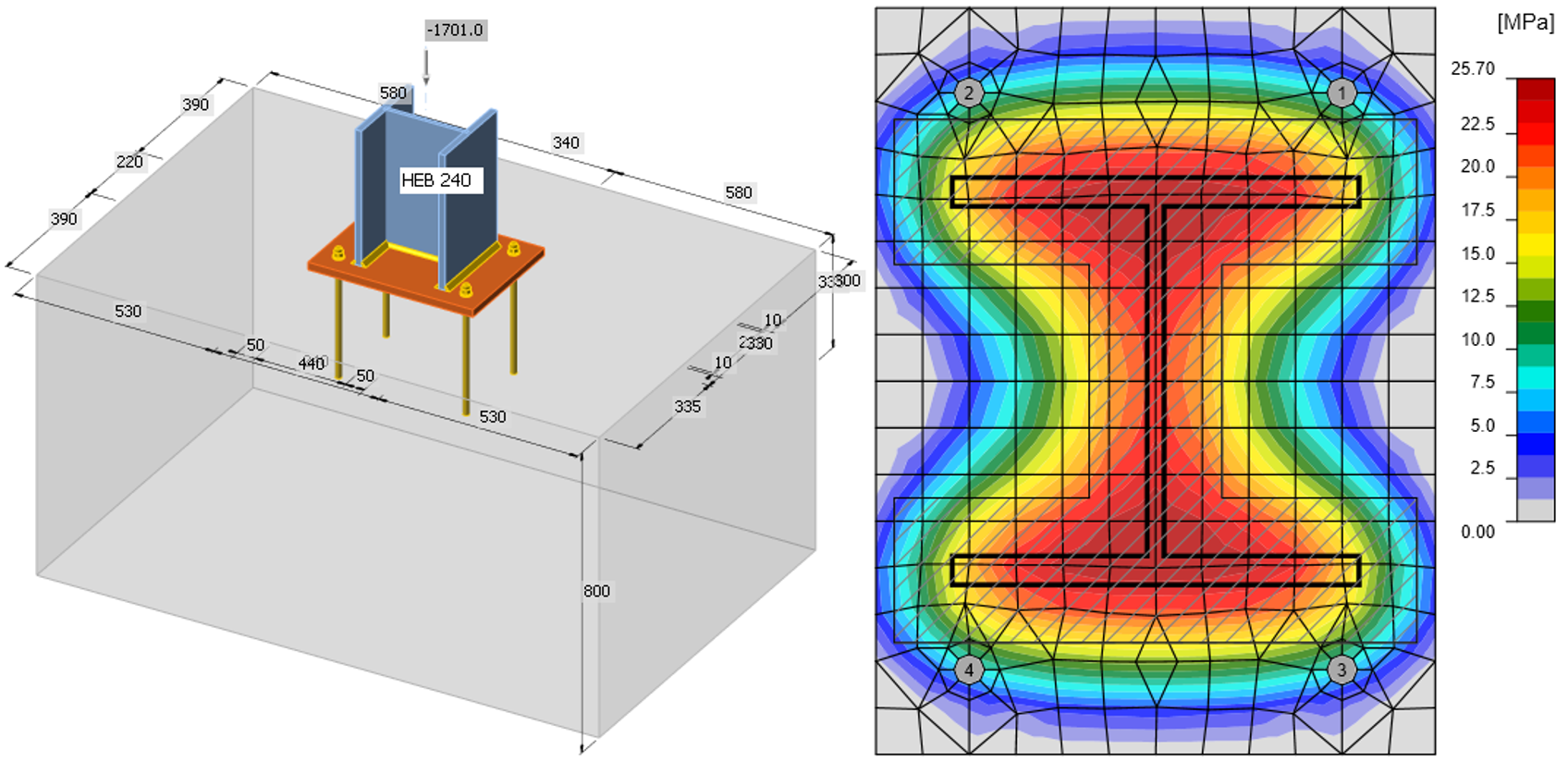
Fig. 8.1.2 Geometria blocului de beton și tensiunile normale sub placa de bază încărcată numai cu forță normală

Studiu de sensibilitate

Rezultatele software-ului CBFEM au fost comparate cu rezultatele metodei componentelor. Comparația a fost axată pe rezistență și componenta critică. Parametrii studiați sunt dimensiunea stâlpului, dimensiunile plăcii de bază, clasa betonului și dimensiunile blocului de beton. Secțiunile transversale ale stâlpului sunt HEB 200, HEB 300 și HEB 400. Lățimea și lungimea plăcii de bază sunt alese cu 100 mm, 150 mm și 200 mm mai mari decât secțiunea stâlpului, grosimea plăcii de bază 15 mm, 20 mm și 25 mm. Blocul de beton din clasa C16/20, C25/30 și C35/45 cu înălțimea de 800 mm, cu lățimea și lungimea mai mari decât dimensiunile plăcii de bază cu 200 mm, 300 mm și 400 mm. Parametrii de intrare sunt rezumați în Tab. 8.1.1. Sudurile de colț în jurul secțiunii transversale a stâlpului au grosimea de gât a = 8 mm.

Tab. 8.1.1 Parametrii selectați

Secțiunea stâlpului	HEB 200	HEB 300	HEB 400
Depășire placă de bază	100 mm	150 mm	200 mm
Grosimea plăcii de bază	15 mm	20 mm	25 mm
Clasa betonului	C16/20	C25/30	C35/45
Depășire bloc de beton	200 mm	300 mm	400 mm

Rezistențele determinate prin MC sunt prezentate în Tab. 8.1.2. Un parametru a fost modificat, iar ceilalți au fost menținuți constanți la valoarea medie. N_Rd este rezistența componentei beton la compresiune inclusiv stratul de nivelare, F_c,fc,Rd este rezistența componentei talpa și inima stâlpului la compresiune, iar F_c,weld este rezistența sudurilor considerând distribuția uniformă a tensiunilor. Coeficientul de îmbinare β_j = 0,67 a fost utilizat.

Tabelul 8.1.2 Rezultatele metodei componentelor

Stâlp	Depășire p.b. [mm]	Grosime p.b. [mm]	Beton	Depășire b.b. [mm]	NRd [kN]	2.Fc,fc,Rd [kN]	Fc,weld [kN]
HEB 200	150	20	C25/30	300	1753	1632	2454
HEB 300	150	20	C25/30	300	2352	3126	3466
HEB 400	150	20	C25/30	300	2579	4040	3822
HEB 300	100	20	C25/30	300	2296	3126	3466
HEB 300	200	20	C25/30	300	2408	3126	3466
HEB 300	150	15	C25/30	300	1909	3126	3466
HEB 300	150	25	C25/30	300	2795	3126	3466
HEB 300	150	20	C16/20	300	1789	3126	3466
HEB 300	150	20	C35/45	300	2908	3126	3466
HEB 300	150	20	C25/30	200	2064	3126	3466
HEB 300	150	20	C25/30	400	2517	3126	3466

Modelul în CBFEM a fost încărcat cu forța de compresiune până când blocul de beton a atins aproape 100 %. Aceeași abordare a fost utilizată pentru a obține rezistența sudurilor F_c,weld.

Tabelul 8.1.3 Rezultatele CBFEM

Stâlp	Depășire p.b. [mm]	Grosime p.b. [mm]	Clasa betonului	Depășire b.b. [mm]	Bloc de beton [kN]	Fc,weld or Fc,Rd [kN]
HEB 200	150	20	C25/30	300	1565	1835
HEB 300	150	20	C25/30	300	2380	3205
HEB 400	150	20	C25/30	300	2710	3650
HEB 300	100	20	C25/30	300	2385	3205
HEB 300	200	20	C25/30	300	2420	3205
HEB 300	150	15	C25/30	300	1870	3204
HEB 300	150	25	C25/30	300	2915	3204
HEB 300	150	20	C16/20	300	1850	3205
HEB 300	150	20	C35/45	300	2975	3205
HEB 300	150	20	C25/30	200	2380	3205
HEB 300	150	20	C25/30	400	2420	3205

Rezumat

Verificarea CBFEM față de MC pentru placa de bază încărcată la compresiune este prezentată în Fig. 8.1.3. Liniile întrerupte corespund valorilor de 110% și 90 % ale rezistenței. Diferența este de până la 14 % datorită evaluării mai precise a rezistenței de calcul la presiune a îmbinării  și a ariei efective  în CBFEM.

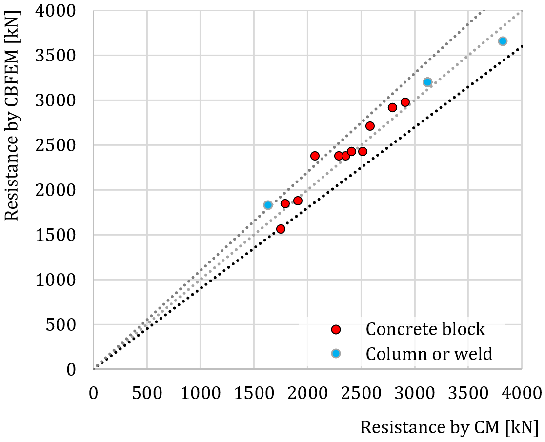
Fig. 8.1.3 Verificarea CBFEM față de MC pentru placa de bază încărcată la compresiune

Caz de referință

Date de intrare

Secțiunea transversală a stâlpului

• HEB 240
• Oțel S235

Placă de bază

• Grosime 20 mm
• Depășiri sus 100 mm, stânga 45 mm
• Oțel S235

Bloc de beton al fundației

• Beton C20/25
• Depășire 335 mm, 530 mm
• Adâncime 800 mm
• Grosime strat de nivelare 30 mm

Buloane de ancorare

• M20 8.8

Rezultate

• Rezistența la forță axială N_j.Rd = −1683 kN

Coloană cu placă de bază – Secțiune deschisă solicitată la încovoiere după axa tare

Descriere

Obiectul acestui capitol este verificarea metodei elementelor finite bazate pe componente (CBFEM) pentru placa de bază a unui stâlp metalic cu secțiune deschisă solicitat la compresiune și încovoiere în jurul axei tari, prin metoda componentelor (CM). Studiul este elaborat pentru dimensiunea stâlpului, geometria și grosimea plăcii de bază. În cadrul studiului, sunt examinate cinci componente: talpa și inima stâlpului la compresiune, betonul la compresiune inclusiv stratul de nivelare, placa de bază la încovoiere, ancorele la întindere și sudurile. Toate componentele sunt proiectate conform EN 1993-1-8:2005, EN 1992‑1‑1:2005 și EN 1992‑4.

Verificarea rezistenței

Un exemplu de proiectare prin metoda componentelor este prezentat pentru ancorarea unui stâlp metalic cu secțiunea HEB 240:

Blocul de beton are dimensiunile a' = 1000 mm, b' = 1500 mm,  h = 900 mm și clasa C20/25. Dimensiunile plăcii de bază sunt a = 330 mm, b = 440 mm, t = 20 mm, iar clasa oțelului este S235. Buloanele de ancorare sunt 4 × M20, A_s = 245 mm², lungime 300 mm, cu diametrul capului a = 60 mm și clasa oțelului 8.8. Grosimea stratului de nivelare este de 30 mm.

Rezultatele soluției analitice pot fi prezentate pe o diagramă de interacțiune cu puncte semnificative distinctive. Punctul −1 reprezintă încărcarea la întindere pură, iar punctul 4 reprezintă rezistența la compresiune. Descrierea detaliată a punctelor 0, 1, 2 și 3 este prezentată în Fig. 8.2.1; a se vedea (Wald, 1995) și (Wald et al. 2008).

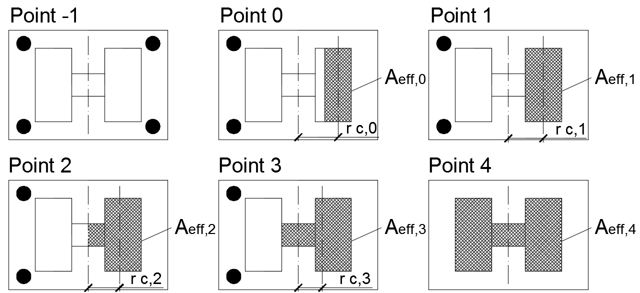
Fig. 8.2.1 Puncte semnificative pe diagrama de interacțiune

Distribuția tensiunilor pentru punctele 0 și 3 obținută prin CBFEM este prezentată în Fig. 8.2.2 și 8.2.3. 

Fig. 8.2.2 Tensiuni în beton și forțe în ancore pentru punctul 0 obținute prin CBFEM (scară deformații 10)

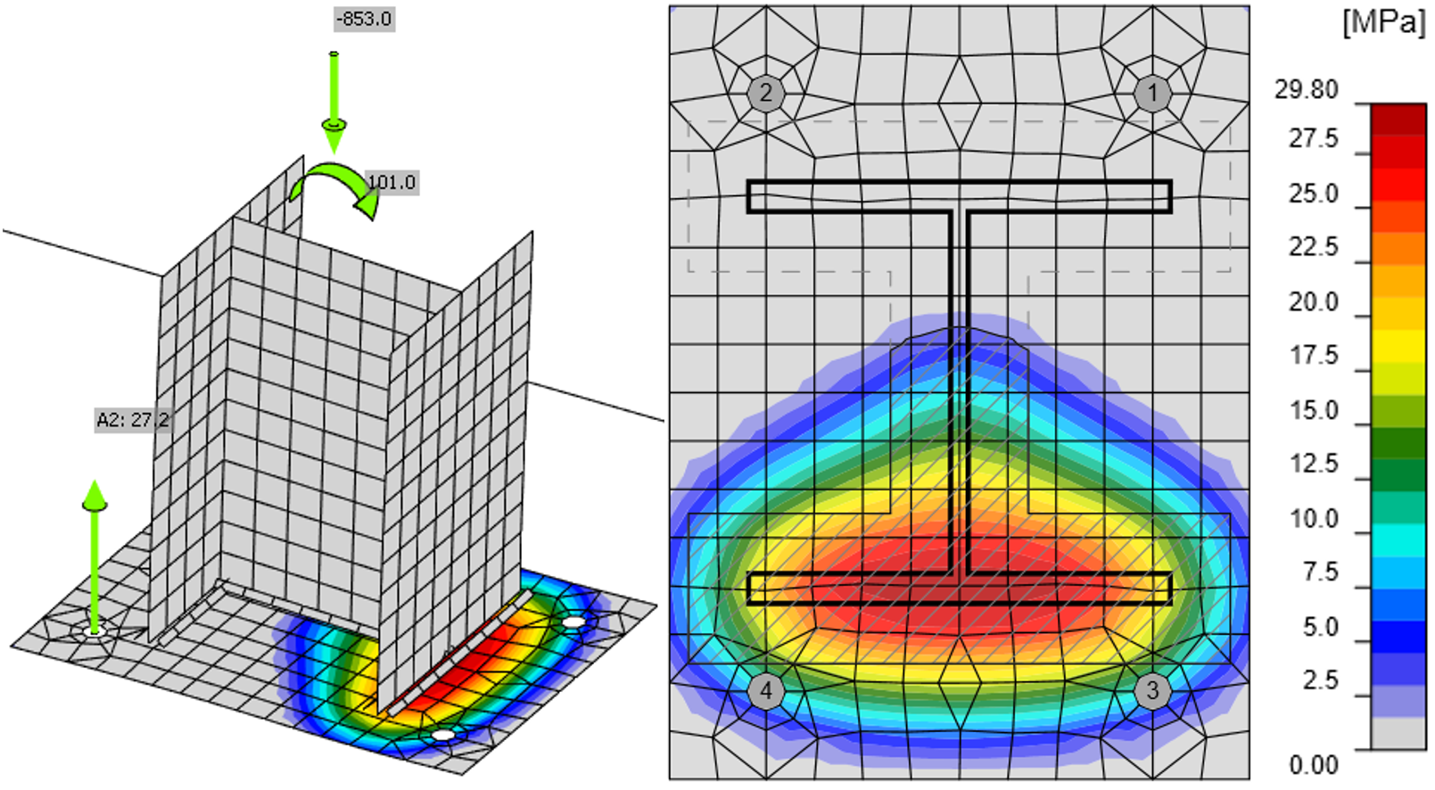
Fig. 8.2.3 Tensiuni în beton și forțe în ancore pentru punctul 3 obținute prin CBFEM
(scară deformații 10)

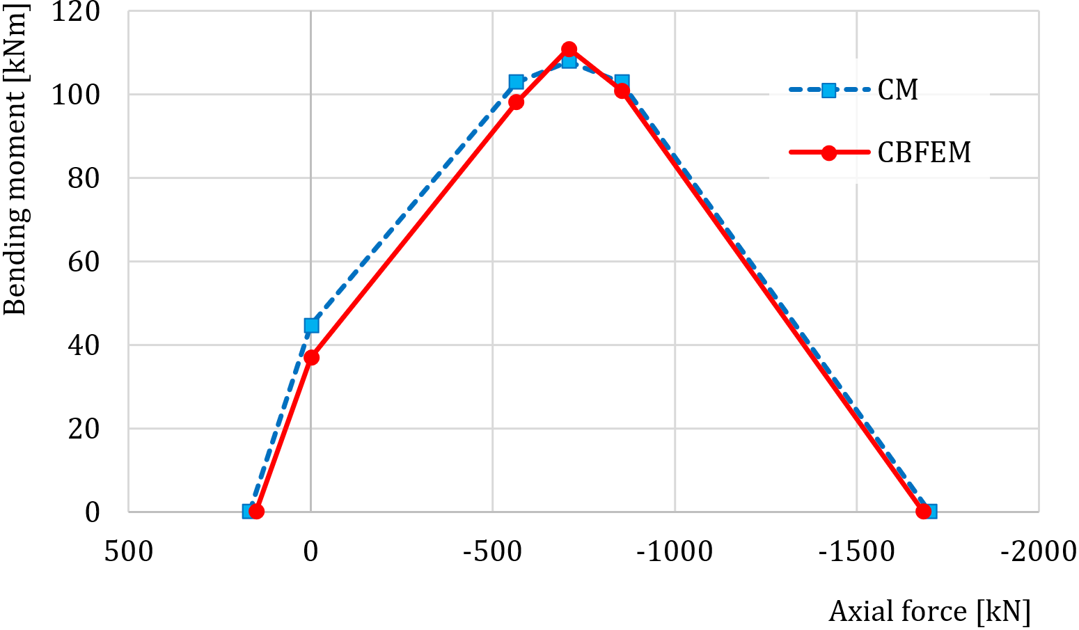
Fig. 8.2.4 Compararea modelelor pe diagrama de interacțiune

Compararea diagramei de interacțiune obținute prin CBFEM cu diagrama de interacțiune calculată conform CM este prezentată în Fig. 8.2.4 și Tab. 8.2.1.

Tab. 8.2.1 Compararea rezultatelor diagramei de interacțiune pentru HEB 240 prin soluție analitică și prin CBFEM

	Soluție analitică		Rezultate CBFEM
	Forță axială  [kN]	Rezistență la încovoiere [kNm]	Forță axială [kN]	Rezistență la încovoiere [kNm]
Punctul -1	169	0	150	0
Punctul 0	0	45	0	37
Punctul 1	−564	103	−564	98
Punctul 2	−708	108	−708	111
Punctul 3	−853	103	−853	101
Punctul 4	−1700	0	−1683	0

Studiu de sensibilitate

Rezultatele CBFEM au fost comparate cu rezultatele metodei componentelor. Compararea a fost realizată prin rezistența la moment încovoietor pentru nivelul dat al forței normale pentru fiecare dintre punctele diagramei de interacțiune.

În studiul de sensibilitate, au fost modificate dimensiunea stâlpului, dimensiunile plăcii de bază și dimensiunile blocului de beton. Secțiunile transversale ale stâlpului selectate au fost HEB 200, HEB 300 și HEB 400. Lățimea și lungimea plăcii de bază au fost alese cu 100 mm, 150 mm și 200 mm mai mari decât secțiunea stâlpului; grosimea plăcii de bază a fost de 15 mm, 20 mm și 25 mm. Blocul de beton a fost din clasa C25/30. Înălțimea blocului de beton a fost în toate cazurile de 900 mm, iar lățimea și lungimea au fost cu 200 mm mai mari decât dimensiunile plăcii de bază. Buloanele de ancorare au fost M20 clasa 8.8 cu o adâncime de încastrare de 300 mm. Parametrii sunt rezumați în Tab. 8.2.2. Sudurile au fost identice pe întregul perimetru al secțiunii stâlpului, cu grosimea de gât suficientă pentru a nu reprezenta componenta critică. Un singur parametru a fost modificat, în timp ce ceilalți au fost menținuți constanți la valoarea medie.

Tab. 8.2.2 Parametrii selectați

Secțiunea stâlpului	HEB 200	HEB 300	HEB 400
Depășire placă de bază	100 mm	150 mm	200 mm
Grosimea plăcii de bază	15 mm	20 mm	25 mm

În Fig. 8.2.5 sunt prezentate rezultatele pentru variațiile secțiunii transversale a stâlpului. În Fig. 8.2.6 și Fig. 8.2.7 sunt variate, respectiv, depășirea plăcii de bază și grosimea plăcii de bază.

Fig. 8.2.5 Variația secțiunii stâlpului

Fig. 8.2.6 Variația depășirii plăcii de bază – 100, 200 și 300 mm

Fig. 8.2.7 Variația grosimii plăcii de bază – 15, 20 și 25 mm

Caz de referință

Date de intrare

Secțiunea transversală a stâlpului

• HEB 240
• Oțel S235

Placă de bază

• Grosime 20 mm
• Depășiri sus 100 mm, stânga 45 mm
• Oțel S235

Bulon de ancorare

• M20 8.8
• Lungime de ancoraj 300 mm
• Tip ancoră: Placă tip șaibă - circulară; dimensiune 40 mm
• Depășiri rânduri superioare 50 mm, rânduri stânga −10 mm
• Plan de forfecare în filet
• Suduri ambele 8 mm

Bloc de fundație

• Beton C20/25
• Depășire 335 mm și 530 mm
• Adâncime 900 mm
• Transfer forță tăietoare prin frecare
• Grosime strat de nivelare 30 mm

Încărcare

• Forță axială N = −853 kN
• Moment încovoietor M_y = 100 kNm

Rezultate

• Buloane de ancorare 42,2 % (N_Ed,g = 51,7 kN ≤ N_Rdc = 122,4 kN - rupere con de beton pentru ancorele A1 și A2)
• Bloc de beton 99,5 % (σ = 26,7 MPa ≤ f_jd = 26,8 MPa)

Referințe

EN 1992-1-1, Eurocode 2, Design of concrete structures – Part 1-1: General rules and rules for buildings, CEN, Brussels, 2005.

EN 1992-4:2018, Eurocode 2: Design of concrete structures – Part 4: Design of fastenings for use in concrete, Brussels, 2018.

EN 1993-1-8, Eurocode 3, Design of steel structures – Part 1-8: Design of joints, CEN, Brussels, 2005.

Wald F. Column Bases, CTU Publishing House, Prague, 1995.

Wald F., Sokol Z., Steenhuis M., Jaspart, J.P. Component method for steel column bases, Heron, 53, 2008, 3-20.

Bază de stâlp – Stâlp cu secțiune tubulară (EN)

Descriere

Metoda elementelor finite bazată pe componente (CBFEM) pentru baza de stâlp cu secțiune tubulară verificată prin metoda componentelor (CM) este descrisă mai jos. Un stâlp comprimat este proiectat cu cel puțin o secțiune transversală de clasa 3. Studiul de sensibilitate este pregătit pentru dimensiunea stâlpului, dimensiunile plăcii de bază, clasa betonului și dimensiunile blocului de beton. Patru componente sunt activate: talpa și inima stâlpului la compresiune, betonul la compresiune inclusiv mortarul de nivelare, ancora la întindere și sudurile. Acest studiu este axat în principal pe două componente: betonul la compresiune inclusiv mortarul de nivelare și ancora la întindere.

Fig. 8.4.1 Puncte semnificative ale diagramei de interacțiune multilineare pentru secțiunea tubulară pătrată

Verificarea rezistenței

În exemplul următor, stâlpul din secțiune tubulară pătrată SHS 150×16 este conectat la blocul de beton cu dimensiunile în plan a' = 750 mm, b' = 750 mm și înălțimea h = 800 mm din beton de clasă C20/25 prin placa de bază a = 350 mm, b = 350 mm, t = 20 mm din oțel S420. Ancore sunt proiectate 4 × M20, A_s = 245 mm² cu diametrul capului a = 60 mm din oțel clasa 8.8 cu decalaje la partea superioară de 50 mm și la stânga de −20 mm și cu adâncimea de încastrare de 300 mm. Mortarul de nivelare are o grosime de 30 mm.

Rezultatele soluției analitice sunt prezentate ca diagramă de interacțiune cu puncte distinctive. O descriere detaliată a punctelor −1, 0, 1, 2 și 3 este prezentată în Fig. 8.4.1; a se vedea (Wald, 1995) și (Wald et al. 2008), unde punctul −1 reprezintă forța de întindere pură, punctul 0 momentul încovoietor pur, punctele 1 până la 3 forța de compresiune combinată cu momentul încovoietor, iar punctul 4 forța de compresiune pură.

Fig.8.4.2 Baza de stâlp pentru stâlpul SHS 150×16 și plasa selectată a plăcii de bază

În CBFEM, efectul de pârghie apare în cazul încărcării la întindere pură; în timp ce în CM, nu se dezvoltă forțe de pârghie prin limitarea rezistenței doar la modul de cedare 1-2; a se vedea (Wald et al. 2008). Datorită efectului de pârghie, diferența de rezistență este de aproximativ 10 %. Modelul numeric al bazei de stâlp este prezentat în Fig. 8.4.2. Rezultatele CBFEM sunt prezentate prin distribuția tensiunilor de contact pe beton pentru punctele 0 și 3, afișate în Fig. 8.4.3 și Fig. 8.4.4, și comparate pe diagrama de interacțiune din Fig. 8.4.5.

Fig. 8.4.3 Rezultate CBFEM pentru punctul 0, adică moment încovoietor pur

Fig. 8.4.4 Rezultate CBFEM pentru punctul 3, adică forță de compresiune și moment încovoietor

Fig. 8.4.5 Compararea rezultatelor predicției rezistenței prin CBFEM și CM pe diagrama de interacțiune pentru baza de stâlp cu secțiunea transversală SHS 150×16

Studiu de sensibilitate

Studiul de sensibilitate este pregătit pentru dimensiunea secțiunii transversale a stâlpului, dimensiunile plăcii de bază, clasa betonului și dimensiunile blocului de beton. Stâlpii selectați sunt SHS 150×16, SHS 160×12.5 și SHS 200×16. Placa de bază este proiectată cu dimensiuni în plan cu 100 mm, 150 mm și 200 mm mai mari decât secțiunea transversală a stâlpului. Grosimea plăcii de bază este de 10 mm, 20 mm și 30 mm. Blocul de fundație este din beton de clasă C20/25, C25/30, C30/37 și C35/45 cu înălțimea de 800 mm pentru toate cazurile și cu dimensiuni în plan cu 100 mm, 200 mm, 300 mm și 500 mm mai mari decât dimensiunile plăcii de bază. Un parametru a fost modificat în timp ce ceilalți au fost menținuți constanți. Parametrii sunt rezumați în Tab. 8.4.1. Sudurile de colț cu grosimea a = 12 mm au fost selectate. Coeficientul de îmbinare pentru mortarul de nivelare de calitate suficientă este luat ca β_j = 0,67. Plăcile de oțel sunt din S420 cu ancore M20 clasa 8.8 cu adâncimea de încastrare de 300 mm în toate cazurile.

Tabelul 8.4.1 Parametrii selectați

Secțiunea transversală a stâlpului	SHS 150×16	SHS 16×12,5	SHS 200×16
Decalaj placă de bază, mm	100	150	200
Grosime placă de bază, mm	10	20	30
Clasa betonului	C20/25	C30/37	C35/45
Decalaj bloc de beton, mm	100	300	500

Pentru studiul de sensibilitate al secțiunii transversale a stâlpului, clasa betonului C20/25, grosimea plăcii de bază de 20 mm, decalajul plăcii de bază de 100 mm și decalajul blocului de beton de 200 mm au fost utilizate pentru varierea parametrilor secțiunii stâlpului. Compararea CBFEM cu modelul analitic prin CM este prezentată în diagramele de interacțiune din Fig. 8.4.6.

Fig. 8.4.6 Compararea rezultatelor CBFEM cu CM pentru diferite secțiuni transversale ale stâlpului

Pentru studiul de sensibilitate al decalajului plăcii de bază, au fost selectate secțiunea transversală a stâlpului SHS 200×16, clasa betonului C25/30, grosimea plăcii de bază de 20 mm și decalajul blocului de beton de 200 mm. Compararea diagramelor de interacțiune este în Fig. 8.4.7. Cea mai semnificativă diferență este în rezistența la întindere pură a unei plăci de bază mari, unde forțe de pârghie semnificative au fost prezente în analizele CBFEM, care sunt limitate prin proiectarea analitică.

Fig. 8.4.7 Compararea rezultatelor CBFEM cu CM pentru diferite decalaje ale plăcii de bază

Pentru studiul de sensibilitate al grosimii plăcii de bază, au fost selectate secțiunea transversală a stâlpului SHS 200×16, clasa betonului C25/30, decalajul plăcii de bază de 100 mm și decalajul blocului de beton de 200 mm. Grosimi ale plăcii de bază de 10 mm, 20 mm și 30 mm au fost utilizate în acest studiu. Compararea diagramelor de interacțiune este în Fig. 8.4.8. Cea mai mare diferență este în rezistența la întindere pură a unei plăci de bază subțiri, unde forțe de pârghie semnificative au fost prezente în analizele CBFEM, care sunt limitate în proiectarea analitică prin CM.

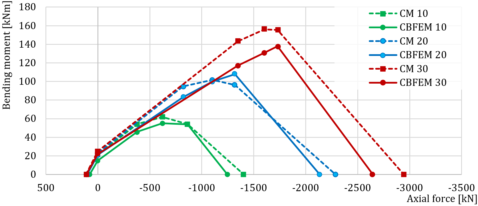
Fig. 8.4.8 Compararea rezultatelor CBFEM cu CM pentru diferite grosimi ale plăcii de bază

Pentru studiul de sensibilitate al clasei betonului, au fost selectate secțiunea transversală a stâlpului SHS 150×16, grosimea plăcii de bază de 20 mm, decalajul plăcii de bază de 100 mm și decalajul blocului de beton de 200 mm. Clasele de beton C20/25, C30/37 și C35/45 au fost utilizate în acest studiu. Compararea diagramelor de interacțiune este în Fig. 8.4.9.

Fig. 8.4.9 Compararea rezultatelor CBFEM cu CM pentru diferite clase de beton

Pentru studiul de sensibilitate al decalajului blocului de beton, au fost selectate secțiunea transversală a stâlpului SHS 160×12.5, grosimea plăcii de bază de 20 mm, decalajul plăcii de bază de 100 mm și clasa betonului C25/30. Decalaje ale blocului de beton de 100 mm, 300 mm și 500 mm au fost utilizate în acest studiu. Compararea diagramelor de interacțiune este în Fig. 8.4.10.

Fig. 8.4.10 Compararea rezultatelor CBFEM cu CM pentru diferite decalaje ale blocului de beton

Diferențele în predicția rezistenței bazei de stâlp prin CBFEM și CM sunt în principal în acceptarea efectului de pârghie în CBFEM și evitarea acestuia prin CM conform EN 1993-1-8:2005.

Tab. 8.4.2 Compararea diagramei de interacțiune CBFEM și CM

Diferență CBFEM/CM	Punctul -1	Punctul 0	Punctul 1	Punctul 2	Punctul 3	Punctul 4
Maximum %	100%	105%	107%	105%	112%	93%
Minimum %	69%	71%	81%	84%	89%	88%

Caz de referință

Date de intrare

Secțiunea transversală a stâlpului

• SHS 150×16
• Oțel S420

Placă de bază

• Grosime 20 mm
• Decalaje la partea superioară 100 mm, la stânga 100 mm
• Suduri – suduri cap la cap
• Oțel S420

Ancore

• M20 8.8.
• Lungime de ancoraj 300 mm
• Tip ancoră: Placă tip șaibă - circulară; dimensiune 40 mm
• Decalaje straturi superioare 50 mm, straturi stânga −20 mm
• Plan de forfecare în filet

Bloc de fundație

• Beton C20/25
• Decalaj 200 mm
• Adâncime 800 mm
• Transfer forță tăietoare prin frecare
• Grosime mortar de nivelare 30 mm

Încărcări

• Forță axială N = −762 kN
• Moment încovoietor M_y = 56 kNm

Rezultate

• Plăci
• Ancore 97,8 % (\(N_{Ed,g} = 65.7 \textrm{ kN} \le N_{Rd,c} = 67.2 \textrm{ kN}\) (componentă critică: smulgerea conului de beton pentru grupul de ancore A1 și A2)
• Bloc de beton 91,5 % (\( \sigma = 24.5 \textrm{ MPa} \le f_{jd} = 26.8 \textrm{ MPa}\))
• Rigiditate rotațională secantă \(S_{js} = 6.3 \textrm{ MNm/rad}\)

Referințe

EN 1993-1-8, Eurocode 3, Proiectarea structurilor de oțel – Partea 1-8: Proiectarea îmbinărilor, CEN, Bruxelles, 2005.

Wald F. Column Bases, CTU Publishing House, Praga, 1995.

Wald F., Sokol Z., Steenhuis M., Jaspart, J.P. Component method for steel column bases, Heron, 53, 2008, 3-20.

Inima stâlpului la forfecare

Îmbinare de colț cu moment încovoietor la streaşină pentru cadru portal sudat

Descriere

În acest capitol, metoda elementelor finite bazată pe componente (CBFEM) pentru o îmbinare de colț cu moment încovoietor la streaşină pentru cadru portal sudat este verificată prin metoda componentelor (CM). O grindă cu secțiune deschisă este sudată la un stâlp cu secțiune deschisă. Stâlpul este rigidizat cu două elemente de rigidizare orizontale opuse tălpilor grinzii. Plăcile comprimate, de ex. elementele de rigidizare orizontale ale stâlpului, panoul inimii stâlpului la forfecare, talpa comprimată a grinzii, sunt limitate la clasa 3^rd pentru a evita flambajul. Căpriorul este încărcat cu forță tăietoare și moment încovoietor.

Model analitic

Cinci componente sunt examinate în studiu, și anume panoul inimii la forfecare, inima stâlpului la compresiune transversală, inima stâlpului la întindere transversală, talpa stâlpului la încovoiere și talpa grinzii la compresiune. Toate componentele sunt proiectate conform EN 1993-1-8:2005. Sudurile de colț sunt proiectate astfel încât să nu fie cea mai slabă componentă a îmbinării. Studiul de verificare al unei suduri de colț într-o îmbinare grindă-stâlp rigidizată se află în capitolul 4.4.

Panoul inimii la forfecare

Grosimea inimii stâlpului este limitată prin zveltețe pentru a evita problemele de stabilitate; a se vedea EN 1993‑1‑8:2005, Cl 6.2.6.1(1). Un panou al inimii stâlpului de clasa 4 la forfecare este studiat în capitolul 6.2. Sunt luate în considerare două contribuții la capacitatea portantă: rezistența panoului stâlpului la forfecare și contribuția mecanismului de cadru al tălpilor stâlpului și al elementelor de rigidizare orizontale; a se vedea EN 1993‑1‑8:2005, Cl. 6.2.6.1 (6.7 și 6.8).

Inima stâlpului la compresiune transversală

Este luată în considerare efectul interacțiunii cu încărcarea de forfecare; a se vedea EN 1993-1-8:2005, Cl. 6.2.6.2, Tab. 6.3. Este luată în considerare influența tensiunii longitudinale în panoul stâlpului; a se vedea EN 1993-1-8:2005, Cl. 6.2.6.2(2). Elementele de rigidizare orizontale sunt incluse în capacitatea portantă a acestei componente.

Inima stâlpului la întindere transversală

Este luată în considerare efectul interacțiunii cu încărcarea de forfecare; a se vedea EN 1993-1-8:2005, Cl. 6.2.6.2, Tab. 6.3. Elementele de rigidizare orizontale sunt incluse în capacitatea portantă a acestei componente.

Talpa stâlpului la încovoiere

Elementele de rigidizare orizontale contravântuiesc talpa stâlpului; această componentă nu este luată în considerare.

Talpa grinzii la compresiune

Grinda orizontală este proiectată să fie de clasa 3 a secțiunii transversale sau mai bună pentru a evita flambajul.

Prezentarea generală a exemplelor considerate și a materialului este dată în Tab. 9.1.1. Geometria îmbinării cu dimensiuni este prezentată în Fig. 9.1.1. Parametrii considerați în studiu sunt secțiunea transversală a grinzii, secțiunea transversală a stâlpului și grosimea panoului inimii stâlpului.

Tab. 9.1.1 Prezentare generală a exemplelor

Exemplu			Material			Grindă	Stâlp	Element de rigidizare stâlp
	fy	fu	E	\(\gamma_{M0}\)	\(\gamma_{M2}\)	Secțiune	Secțiune	bs	ts
	[MPa]	[MPa]	[GPa]	[-]	[-]			[mm]	[mm]
IPE140	235	360	210	1	1,25	IPE140	HEB260	73	10
IPE160	235	360	210	1	1,25	IPE160	HEB260	82	10
IPE180	235	360	210	1	1,25	IPE180	HEB260	91	10
IPE200	235	360	210	1	1,25	IPE200	HEB260	100	10
IPE220	235	360	210	1	1,25	IPE220	HEB260	110	10
IPE240	235	360	210	1	1,25	IPE240	HEB260	120	10
IPE270	235	360	210	1	1,25	IPE270	HEB260	135	10
IPE300	235	360	210	1	1,25	IPE300	HEB260	150	10
IPE330	235	360	210	1	1,25	IPE330	HEB260	160	10
IPE360	235	360	210	1	1,25	IPE360	HEB260	170	10
IPE400	235	360	210	1	1,25	IPE400	HEB260	180	10
IPE450	235	360	210	1	1,25	IPE450	HEB260	190	10
IPE500	235	360	210	1	1,25	IPE500	HEB260	200	10

Exemplu			Material			Grindă	Stâlp	Element de rigidizare stâlp
	fy	fu	E	\(\gamma_{M0}\)	\(\gamma_{M2}\)	Secțiune	Secțiune	bs	ts
	[MPa]	[MPa]	[GPa]	[-]	[-]			[mm]	[mm]
HEB160	235	360	210	1	1,25	IPE330	HEB160	160	10
HEB180	235	360	210	1	1,25	IPE330	HEB180	160	10
HEB200	235	360	210	1	1,25	IPE330	HEB200	160	10
HEB220	235	360	210	1	1,25	IPE330	HEB220	160	10
HEB240	235	360	210	1	1,25	IPE330	HEB240	160	10
HEB260	235	360	210	1	1,25	IPE330	HEB260	160	10
HEB280	235	360	210	1	1,25	IPE330	HEB280	160	10
HEB300	235	360	210	1	1,25	IPE330	HEB300	160	10
HEB320	235	360	210	1	1,25	IPE330	HEB320	160	10
HEB340	235	360	210	1	1,25	IPE330	HEB340	160	10
HEB360	235	360	210	1	1,25	IPE330	HEB360	160	10
HEB400	235	360	210	1	1,25	IPE330	HEB400	160	10
HEB500	235	360	210	1	1,25	IPE330	HEB500	160	10

Exemplu			Material			Grindă	Stâlp		Element de rigidizare stâlp
	fy	fu	E	\(\gamma_{M0}\)	\(\gamma_{M2}\)	Secțiune	Secțiune	tw	bs	ts
	[MPa]	[MPa]	[GPa]	[-]	[-]			[mm]	[mm]	[mm]
tw4	235	360	210	1	1,25	IPE330	HEA320	4	160	10
tw5	235	360	210	1	1,25	IPE330	HEA320	5	160	10
tw6	235	360	210	1	1,25	IPE330	HEA320	6	160	10
tw7	235	360	210	1	1,25	IPE330	HEA320	7	160	10
tw8	235	360	210	1	1,25	IPE330	HEA320	8	160	10
tw9	235	360	210	1	1,25	IPE330	HEA320	9	160	10
tw10	235	360	210	1	1,25	IPE330	HEA320	10	160	10
tw11	235	360	210	1	1,25	IPE330	HEA320	11	160	10
tw12	235	360	210	1	1,25	IPE330	HEA320	12	160	10
tw13	235	360	210	1	1,25	IPE330	HEA320	13	160	10
tw14	235	360	210	1	1,25	IPE330	HEA320	14	160	10
tw15	235	360	210	1	1,25	IPE330	HEA320	15	160	10

\[ \textsf{\textit{\footnotesize{Fig. 9.1.1 Geometria și dimensiunile îmbinării}}}\]

Model numeric

Starea materialului elastic-plastic neliniară este investigată în fiecare strat al unui punct de integrare. Evaluarea se bazează pe deformația maximă dată conform EN 1993-1-5:2006 prin valoarea de 5%. 

Comportament global

Este prezentată comparația comportamentului global al unei îmbinări cu moment încovoietor pentru cadru portal, descrisă prin diagrama moment-rotație. Caracteristicile principale ale diagramei moment-rotație sunt rigiditatea inițială, rezistența elastică și rezistența de calcul. O grindă cu secțiune deschisă IPE 330 este sudată la un stâlp HEB 260 în exemplu. O îmbinare cu moment încovoietor pentru cadru portal cu elemente de rigidizare orizontale în stâlp este considerată conform metodei componentelor ca un rost rigid cu S_j,ini = ∞. Prin urmare, este analizată o îmbinare fără elemente de rigidizare orizontale în stâlp. Diagrama moment-rotație este prezentată în Fig. 9.1.2, iar rezultatele sunt rezumate în Tab. 9.1.2. Rezultatele arată o concordanță foarte bună în rigiditatea inițială și comportamentul global al îmbinării.

Tab. 9.1.2 Rigiditatea de rotație a unei îmbinări cu moment încovoietor pentru cadru portal în CBFEM și CM

		CM	CBFEM	CM/CBFEM
Rigiditate inițială Sj,ini	[kNm/rad]	48423,7	58400,0	0,83
Rezistență elastică 2/3 Mj,Rd	[kNm]	93,3	93,0	1,00
Rezistență de calcul Mj,Rd	[kNm]	140,0	139,0	0,99

\[ \textsf{\textit{\footnotesize{Fig. 9.1.2 Diagrama moment-rotație pentru o îmbinare fără elemente de rigidizare ale stâlpului}}}\]

Verificarea rezistenței

Rezultatele calculate prin CBFEM sunt comparate cu CM. Comparația este axată pe rezistența de calcul și componenta critică. Studiul este realizat pentru trei parametri diferiți: secțiunea transversală a grinzii, secțiunea transversală a stâlpului și grosimea panoului inimii stâlpului.

Un stâlp cu secțiune deschisă HEB 260 este utilizat într-un exemplu în care parametrul este secțiunea transversală a grinzii. Stâlpul este rigidizat cu două elemente de rigidizare orizontale ale stâlpului cu grosimea de 10 mm opuse tălpilor grinzii. Lățimea elementelor de rigidizare corespunde lățimii tălpii grinzii. Secțiunile IPE ale grinzii sunt selectate de la IPE 140 la IPE 500. Rezultatele sunt prezentate în Tab. 9.1.3. Influența secțiunii transversale a grinzii asupra rezistenței de calcul a unei îmbinări cu moment încovoietor pentru cadru portal sudat este prezentată în Fig. 9.1.4. Componentele critice în CBFEM au fost tălpile grinzii, talpa stâlpului și inima stâlpului. Fig. 9.1.3. prezintă modelul unuia dintre exemple cu descrierea tălpilor. 

\[ \textsf{\textit{\footnotesize{Fig. 9.1.3 Model cu descrierea tălpilor}}}\]

Tab. 9.1.3 Rezistențe de calcul și componente critice în CBFEM și CM

\[ \textsf{\textit{\footnotesize{Fig. 9.1.4 Studiu de sensibilitate al dimensiunii grinzii într-o îmbinare cu moment încovoietor pentru cadru portal}}}\]

O grindă cu secțiune deschisă IPE330 este utilizată într-un exemplu în care parametrul este secțiunea transversală a stâlpului. Stâlpul este rigidizat cu două elemente de rigidizare orizontale ale stâlpului cu grosimea de 10 mm opuse tălpilor grinzii. Lățimea elementelor de rigidizare corespunde lățimii tălpii grinzii. Lățimea combinată a elementelor de rigidizare este de 160 mm. Secțiunile stâlpului sunt selectate de la HEB 160 la HEB 500. Rezultatele sunt prezentate în Tab. 9.1.4. Influența secțiunii transversale a stâlpului asupra rezistenței de calcul a unei îmbinări cu moment încovoietor pentru cadru portal sudat este prezentată în Fig. 9.1.5.

Tab. 9.1.4 Rezistențe de calcul și componente critice ale unei îmbinări cu moment încovoietor în CBFEM și CM

\[ \textsf{\textit{\footnotesize{Fig. 9.1.5 Studiu de sensibilitate al dimensiunii stâlpului într-o îmbinare cu moment încovoietor pentru cadru portal}}}\]

Al treilea exemplu prezintă o îmbinare cu moment încovoietor pentru cadru portal alcătuită dintr-o grindă cu secțiune deschisă IPE 330 și stâlp HEA 320. Parametrul este grosimea inimii stâlpului. Stâlpul este rigidizat cu două elemente de rigidizare orizontale ale stâlpului cu grosimea de 10 mm și lățimea de 160 mm. Grosimea inimii stâlpului este aleasă de la 4 la 16 mm. Rezultatele sunt rezumate în Tab. 9.1.5. Influența grosimii inimii stâlpului asupra rezistenței de calcul a unei îmbinări cu moment încovoietor pentru cadru portal sudat este prezentată în Fig. 9.1.6.

Tab. 9.1.5 Rezistențe de calcul și componente critice ale unei îmbinări cu moment încovoietor în CBFEM și CM

\[ \textsf{\textit{\footnotesize{Fig. 9.1.6 Studiu de sensibilitate al grosimii inimii stâlpului}}}\]

Pentru a ilustra acuratețea modelului CBFEM, rezultatele studiilor parametrice sunt rezumate într-o diagramă care compară rezistențele CBFEM și ale metodei componentelor; a se vedea Fig. 9.1.7. Rezultatele arată că diferența dintre cele două metode de calcul este mai mică de 5%, ceea ce reprezintă o valoare general acceptabilă. Studiul cu parametrul grosimea inimii stâlpului oferă o rezistență mai mare pentru modelul CBFEM comparativ cu metoda componentelor. Această diferență este cauzată de luarea în considerare a secțiunilor sudate. Transferul încărcării de forfecare este considerat în metoda componentelor doar în inimă, iar contribuția tălpilor este neglijată.

\[ \textsf{\textit{\footnotesize{Fig. 9.1.7 Verificarea CBFEM față de CM}}}\]

Exemplu de referință

Date de intrare

Stâlp

• Oțel S235
• HEB260

Grindă

• Oțel S235
• IPE330

Elemente de rigidizare stâlp

• Grosime t_s = 19 mm
• Lățime 80 mm
• Opuse tălpilor grinzii

Sudură

• Talpa grinzii: grosimea gâtului sudurii de colț a_f  = 8 mm
• Inima grinzii: grosimea gâtului sudurii de colț a_w  = 8 mm
• Sudură cap la cap în jurul elementelor de rigidizare

Rezultate

• Rezistența de calcul la încovoiere M_Rd = 146 kNm
• Componentă critică: Talpa grinzii 1

\[ \textsf{\textit{\footnotesize{Fig. 9.1.8 Exemplu de referință}}}\]

Îmbinare cu moment la streașina unui cadru portal cu șuruburi

Descriere

Obiectivul acestui studiu este verificarea îmbinării cu moment la streașina unui cadru portal cu șuruburi, așa cum se arată în Fig. 9.2.1. Căpriorul este prins cu șuruburi prin placă de capăt pe talpa stâlpului. Stâlpul este rigidizat cu două elemente de rigidizare orizontale la nivelul tălpilor grinzii. Plăcile comprimate, de ex. elementele de rigidizare orizontale ale stâlpului, panoul inimii la forfecare sau compresiune și talpa comprimată a grinzii, sunt proiectate ca secțiuni transversale de clasa 3. Grinda orizontală are 6 m lungime și este încărcată cu o încărcare continuă pe întreaga lungime.

Fig. 9.2.1 Îmbinare cu moment la streașina unui cadru portal cu șuruburi

Model analitic

Sunt examinate opt componente: sudură de colț, panoul inimii la forfecare, inima stâlpului la compresiune transversală, inima stâlpului la întindere transversală, talpa grinzii la compresiune și întindere, talpa stâlpului la încovoiere, placa de capăt la încovoiere și șuruburi. Toate componentele sunt proiectate conform EN 1993-1-8:2005. Valorile de calcul ale încărcărilor pe componente depind de poziție. Panoul inimii la forfecare este încărcat cu valorile de calcul ale încărcărilor pe axa verticală a stâlpului. Celelalte componente sunt încărcate cu valorile de calcul reduse ale încărcărilor în talpa stâlpului la care este conectată grinda orizontală.

Sudură de colț

Sudura este continuă pe întregul perimetru al secțiunii transversale a grinzii. Grosimea sudurii pe tălpi poate diferi de grosimea sudurii pe inimă. Forța tăietoare verticală este transferată numai prin sudurile de pe inimă, considerându-se o distribuție plastică a tensiunilor. Momentul încovoietor este transferat prin întreaga formă a sudurii, considerându-se o distribuție elastică a tensiunilor. Se ia în considerare lățimea efectivă a sudurii în funcție de rigiditatea orizontală a stâlpului (datorită încovoierii tălpii nestifenizate a stâlpului). Proiectarea sudurii se face conform EN 1993-1-8:2005, Cl. 4.5.3.2(6). Verificarea se efectuează în două puncte principale: pe muchia superioară sau inferioară a tălpii (tensiune maximă de încovoiere) și la intersecția tălpii cu inima (combinație de tensiuni din forță tăietoare și moment încovoietor).

Panoul inimii la forfecare

Grosimea inimii stâlpului este proiectată să fie cel mult de clasa a treia; a se vedea EN 1993-1-8:2005, Cl. 6.2.6.1(1). Se iau în considerare două contribuții la capacitatea portantă: rezistența peretelui stâlpului la forfecare și contribuția din comportarea de cadru a tălpilor stâlpului și a elementelor de rigidizare orizontale; a se vedea EN 1993-1-8:2005, Cl. 6.2.6.1 (6.7 și 6.8).

Inima stâlpului la compresiune sau întindere transversală

Se ia în considerare efectul interacțiunii cu încărcarea de forfecare; a se vedea EN 1993-1-8:2005, Cl. 6.2.6.2 și Tab. 6.3. Se ia în considerare influența tensiunii longitudinale din peretele stâlpului; a se vedea EN 1993-1-8:2005, Cl. 6.2.6.2(2). Elementele de rigidizare orizontale previn flambajul și sunt incluse în capacitatea portantă a acestei componente cu aria efectivă.

Talpa grinzii la compresiune

Grinda orizontală este proiectată să fie cel mult de clasa a treia.

Talpa stâlpului sau placa de capăt la încovoiere

Lungimile efective pentru cedările circulare și necirculare sunt considerate conform EN 1993-1-8:2005, Cl. 6.2.6. Sunt considerate trei moduri de cedare conform EN 1993-1-8:2005, Cl. 6.2.4.1.

Șuruburi

Șuruburile sunt proiectate conform EN 1993-1-8:2005, Cl. 3.6.1. Rezistența de calcul ia în considerare rezistența la forfecare prin poansonare și ruperea șurubului.

Model numeric de calcul

Grinda T este modelată cu elemente de tip placă cu 4 noduri, așa cum este descris în Capitolul 3 și rezumat în continuare. Fiecare nod are 6 grade de libertate. Deformațiile elementului constau din contribuții membranare și de încovoiere. Starea elastoplastică neliniară a materialului este investigată în fiecare strat al punctului de integrare. Verificarea se bazează pe deformația maximă dată conform EN 1993-1-5:2006 prin valoarea de 5 %. Șuruburile sunt împărțite în trei sub-componente. Prima este tija șurubului, modelată ca un arc neliniar care preia numai întindere. A doua sub-componentă transmite forța de întindere în tălpi. A treia sub-componentă rezolvă transmiterea forței tăietoare.

Comportare globală

S-a realizat compararea comportării globale a îmbinării, descrisă prin diagrame moment-rotație pentru ambele proceduri de calcul menționate mai sus. Atenția a fost concentrată pe caracteristicile principale ale diagramei moment-rotație: rigiditate inițială, rezistență de calcul și capacitate de deformare. Grinda IPE 330 este conectată la stâlpul HEB 300 prin placă de capăt extinsă cu 5 rânduri de șuruburi M24 8.8. Rezultatele ambelor proceduri de calcul sunt prezentate în graficul din Fig. 9.2.2 și în Tab. 9.2.1. Metoda componentelor (CM) oferă în general o rigiditate inițială mai mare comparativ cu CBFEM. CBFEM oferă o rezistență de calcul ușor mai mare comparativ cu CM în toate cazurile, așa cum se arată în Capitolul 9.2.5. Diferența este de până la 10%. Capacitatea de deformare este de asemenea comparată. Capacitatea de deformare a fost calculată conform (Beg et al. 2004), deoarece EC3 oferă o bază limitată pentru capacitatea de deformare a îmbinărilor cu placă de capăt.

Fig. 9.2.2 Diagramă moment-rotație

Tab. 9.2.1 Prezentare generală a comportării globale

		CM	CBFEM	CM/CBFEM
Rigiditate inițială	[kNm/rad]	67400	112000	0,60
Rezistență de calcul	[kNm]	204	199	0,98
Capacitate de deformare	[mrad]	242	47	5,14

Verificarea rezistenței

Rezistența de calcul calculată prin CBFEM a fost comparată cu rezultatele metodei componentelor în etapa următoare. Comparația s-a concentrat atât pe rezistență, cât și pe componenta critică. Studiul a fost realizat pentru parametrul secțiunii transversale a stâlpului. Grinda IPE 330 este conectată la stâlp prin placă de capăt extinsă cu 5 rânduri de șuruburi. Se utilizează șuruburi M24 8.8. Dimensiunile plăcii de capăt P15 cu distanțele marginale și spațierile șuruburilor în milimetri sunt: înălțimea 450 (50-103-75-75-75-73) și lățimea 200 (50-100-50). Muchia exterioară a tălpii superioare se află la 91 mm de marginea plăcii de capăt. Tălpile grinzii sunt conectate la placa de capăt cu suduri cu grosimea de gât de 8 mm. Inima grinzii este conectată cu grosimea de gât a sudurii de 5 mm. Stâlpul este rigidizat cu elemente de rigidizare orizontale în dreptul tălpilor grinzii. Elementele de rigidizare au grosimea de 15 mm, iar lățimea lor corespunde lățimii stâlpului. Grosimea elementului de rigidizare al plăcii de capăt este de 10 mm, iar lățimea sa este de 90 mm. Rezultatele sunt prezentate în Tab. 9.2.2 și Fig. 9.2.3.

Tab. 9.2.2 Rezistența de calcul pentru parametru – profil stâlp

Secțiunea transversală a stâlpului	CM		CBFEM		CM/ CBFEM
	Rezistență	Componentă	Rezistență	Componentă
	[kNm]		[kNm]
HEB 200	107	Inima stâlpului la forfecare	106	Inima stâlpului la forfecare	1,01
HEB 220	121	Inima stâlpului la forfecare	136	Inima stâlpului la forfecare	0,89
HEB 240	143	Inima stâlpului la forfecare	155	Inima stâlpului la forfecare	0,92
HEB 260	160	Inima stâlpului la forfecare	169	Inima stâlpului la forfecare	0,95
HEB 280	176	Inima stâlpului la forfecare	187	Inima stâlpului la forfecare	0,94
HEB 300	204	Inima stâlpului la forfecare	199	Talpa grinzii la întindere/compresiune	0,98
HEB 320	222	Inima stâlpului la forfecare	225	Talpa grinzii la întindere/compresiune	0,99
HEB 340	226	Talpa grinzii la întindere/compresiune	242	Talpa grinzii la întindere/compresiune	0,93
HEB 360	229	Talpa grinzii la întindere/compresiune	239	Talpa grinzii la întindere/compresiune	0,96
HEB 400	234	Talpa grinzii la întindere/compresiune	253	Talpa grinzii la întindere/compresiune	0,92
HEB 450	241	Talpa grinzii la întindere/compresiune	260	Talpa grinzii la întindere/compresiune	0,93
HEB 500	248	Talpa grinzii la întindere/compresiune	268	Talpa grinzii la întindere/compresiune	0,93

Fig. 9.2.3 Rezistența de calcul în funcție de secțiunea transversală a stâlpului

Pentru a ilustra acuratețea modelului CBFEM, rezultatele studiilor parametrice sunt rezumate în graficul care compară rezistențele estimate de CBFEM și de CM; a se vedea Fig. 9.2.4. Rezultatele arată că CBFEM oferă o rezistență de calcul ușor mai mare comparativ cu CM în aproape toate cazurile. Diferența dintre cele două metode este de până la 10%.

Fig. 9.2.4 Verificarea CBFEM față de CM

Exemplu de referință

Date de intrare

• Oțel S235
• Grindă IPE 330
• Stâlp HEB 300
• Înălțimea plăcii de capăt h_p = 450 (50-103-75-75-75-73) mm
• Lățimea plăcii de capăt b_p = 200 (50-100-50) mm
• Placă de capăt P15
• Elemente de rigidizare ale stâlpului cu grosimea de 15 mm și lățimea de 300 mm
• Element de rigidizare al plăcii de capăt cu grosimea de 10 mm, lățimea și înălțimea de 90 mm, muchii teșite de 20 mm 
• Grosimea de gât a sudurii tălpii a_f = 8 mm
• Grosimea de gât a sudurii inimii și a elementului de rigidizare al plăcii de capăt a_w = 5 mm
• Șuruburi M24 8.8

Rezultate

• Rezistența de calcul la încovoiere M_Rd = 206 kNm
• Forța tăietoare verticală corespunzătoare V_Ed= –206 kN
• Mod de cedare: curgerea elementului de rigidizare al grinzii pe talpa superioară
• Gradul de utilizare al șuruburilor 90,2 %
• Gradul de utilizare al sudurilor 99,0 %

Predicția rigidității

Rigiditatea la încovoiere a îmbinării sudate a secțiunilor deschise

Descriere

Predicția rigidității de rotație este descrisă pe o îmbinare sudată de colț cu moment încovoietor. Se studiază o îmbinare sudată a unui stâlp cu secțiune deschisă HEB și a unei grinzi IPE, iar comportamentul îmbinării este descris printr-o diagramă moment-rotație. Rezultatele modelului analitic prin metoda componentelor (CM) sunt comparate cu rezultatele numerice obținute prin metoda elementelor finite bazată pe componente (CBFEM). Este disponibil un caz de referință.

Model analitic

Rigiditatea de rotație a unei îmbinări trebuie determinată din deformația componentelor sale de bază, care sunt reprezentate prin coeficientul de rigiditate k_i. Rigiditatea de rotație a îmbinării S_j se obține din:

\[ S_j = \frac{E z^2}{\mu \Sigma_i \frac{1}{k_i}} \]

unde:

• k_i  este coeficientul de rigiditate pentru componenta i a îmbinării;
• z   este brațul de pârghie; a se vedea 6.2.7;
• μ   este raportul de rigiditate; a se vedea 6.3.1.

Componentele îmbinării luate în considerare în acest exemplu sunt panoul inimii stâlpului la forfecare k₁, inima stâlpului la compresiune k_2, și inima stâlpului la întindere k₃. Coeficienții de rigiditate sunt definiți în Tabelul 6.11 din EN 1993-1-8:2005. Rigiditatea inițială S_j,ini se obține pentru un moment M_j,Ed ≤ 2/3 M_j,Rd.

\[S_j = \frac{E \, z^{2}}{\frac{1}{k_1} + \frac{1}{k_2} + \frac{1}{k_3}}\]

\[S_{j,\text{ini}} = \frac{S_j}{1.5^{\psi}}\]

unde 

\(S_{j}\) — rigiditatea de rotație a îmbinării

\(\psi\) = 2,7 — EN 1993-1-8 tabelul 6.8

În exemplu, o grindă cu secțiune deschisă IPE 400 este sudată la un stâlp HEB 300. Tălpile grinzii sunt conectate la talpa stâlpului prin suduri cu grosimea de calcul a cordonului de 9 mm. Inima grinzii este conectată prin suduri cu grosimea de calcul a cordonului de 5 mm. Se consideră distribuția plastică a tensiunilor în suduri. Materialul grinzii și al stâlpului este S235. Rezistența de calcul este limitată de componentele panoul stâlpului la forfecare și panoul stâlpului la compresiune transversală. Coeficienții de rigiditate calculați ai componentelor de bază, rigiditatea inițială, rigiditatea la rezistența de calcul și rotația grinzii sunt rezumate în Tab. 10.1.1.

\[ \textsf{\textit{\footnotesize{Tab. 10.1.1 Rezultatele modelului analitic}}}\]

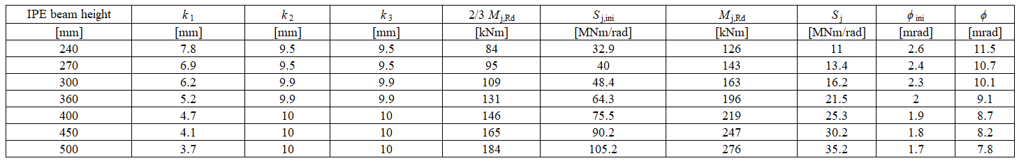
Model numeric

Informații detaliate despre predicția rigidității în CBFEM pot fi găsite în capitolul 3.9. Aceeași îmbinare sudată de colț cu moment încovoietor este modelată, iar rezultatele sunt prezentate în Tab. 10.1.2. Rezistența de calcul este atinsă la o deformație plastică de 5% în componenta inima stâlpului la întindere. Analizele CBFEM permit calculul rigidității de rotație în orice etapă de încărcare.

Prezentare generală experimentală 

În scopul comparației, secțiunea transversală a stâlpului a fost stabilită la HEB300, iar secțiunea transversală a grinzii a fost variabilă. Toate materialele utilizate au fost S235. 

\[ \textsf{\textit{\footnotesize{Tab. 10.1.2 Prezentare generală experimentală}}}\]

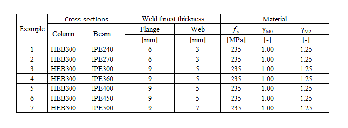
\[ \textsf{\textit{\footnotesize{Tab. 10.1.3 Prezentare generală experimentală}}}\]

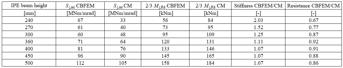
\[ \textsf{\textit{\footnotesize{Fig. 1 Verificarea CBFEM față de CM}}}\]

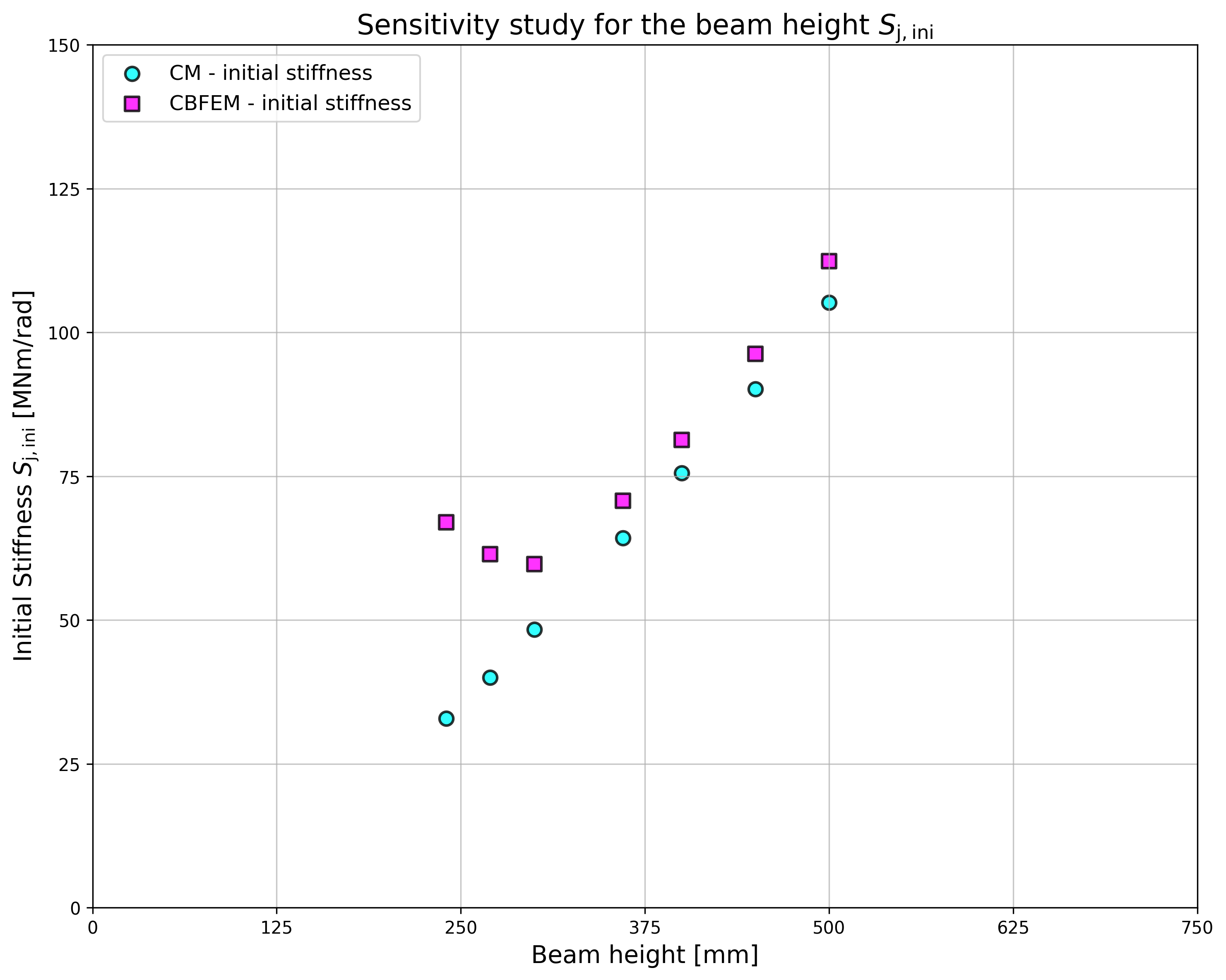
\[ \textsf{\textit{\footnotesize{Fig. 2 Studiu de sensibilitate al secțiunii transversale a grinzii IPE}}}\]

Verificarea rigidității

Rigiditatea de rotație calculată prin CBFEM este comparată cu CM. Comparația arată o bună concordanță a rigidității inițiale și corespondența comportamentului îmbinării. Rigiditatea calculată prin CBFEM și CM este rezumată în Tab. 10.1.3.

Este pregătită o comparație a comportamentului global al unei îmbinări sudate de colț cu moment încovoietor, descrisă printr-o diagramă moment-rotație. Îmbinarea este analizată și se calculează rigiditatea grinzii conectate. Caracteristica principală este rigiditatea inițială calculată la 2/3M_j,Rd, unde M_j,Rd este rezistența de calcul la moment a îmbinării. Diagrama moment-rotație este prezentată în Fig. 10.1.1.

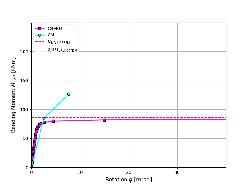
\[ \textsf{\textit{\footnotesize{Fig. 3 Diagrama moment-rotație pentru o îmbinare sudată de colț cu moment încovoietor, IPE240}}}\]

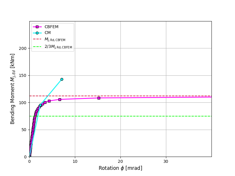
\[ \textsf{\textit{\footnotesize{Fig. 4 Diagrama moment-rotație pentru o îmbinare sudată de colț cu moment încovoietor, IPE270}}}\]

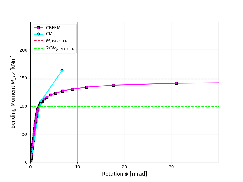
\[ \textsf{\textit{\footnotesize{Fig. 5 Diagrama moment-rotație pentru o îmbinare sudată de colț cu moment încovoietor, IPE300}}}\]

\[ \textsf{\textit{\footnotesize{Fig. 6 Diagrama moment-rotație pentru o îmbinare sudată de colț cu moment încovoietor, IPE360}}}\]

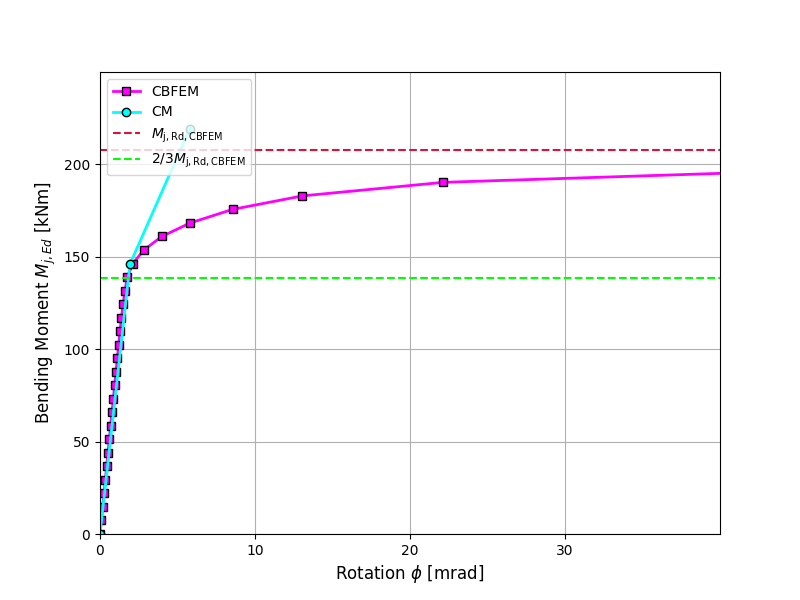
\[ \textsf{\textit{\footnotesize{Fig. 7 Diagrama moment-rotație pentru o îmbinare sudată de colț cu moment încovoietor, IPE400}}}\]

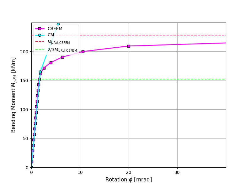
\[ \textsf{\textit{\footnotesize{Fig. 8 Diagrama moment-rotație pentru o îmbinare sudată de colț cu moment încovoietor, IPE450}}}\]

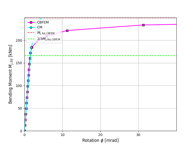
\[ \textsf{\textit{\footnotesize{Fig. 9 Diagrama moment-rotație pentru o îmbinare sudată de colț cu moment încovoietor, IPE500}}}\]

Caz de referință

Date de intrare

Grindă și stâlp

• Oțel S235
• Stâlp HEB 300
• Grindă IPE 400
• Grosimea de calcul a cordonului de sudură la talpă a_f  = 9 mm
• Grosimea de calcul a cordonului de sudură la inimă a_w  = 5 mm
• Excentricitatea stâlpului s = 150 mm
• Sudură de colț dublă

Date de ieșire

• Rezistența de calcul \(M_\mathrm{j,Rd}= 199 \quad \mathrm{kNm}\)
• Încărcarea \(M_\mathrm{j,Ed}=2/3M_\mathrm{j,Rd}= 133\quad \mathrm{kNm}\) 
• Rigiditatea de rotație secantă \(S_\mathrm{j,ini}= 81.3\quad \mathrm{MNm/rad}\) 

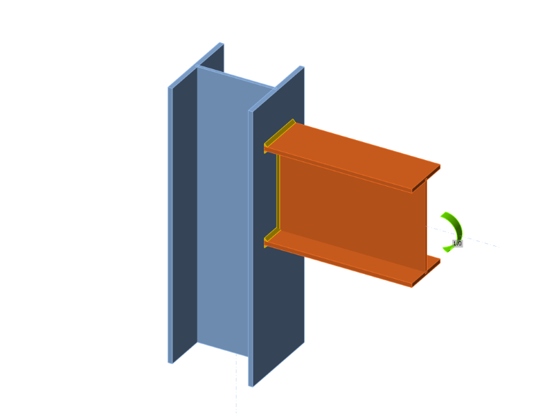
\[ \textsf{\textit{\footnotesize{Fig. 10 Caz de referință pentru îmbinarea sudată de colț cu moment încovoietor (IPE 400 la HEB 300)}}}\]

Rigiditatea la încovoiere a îmbinării cu șuruburi a secțiunilor deschise

10.2.1 Descriere

Predicția rigidității de rotație este verificată pe o îmbinare cu moment la streașină cu șuruburi. Se studiază o îmbinare cu șuruburi a unui stâlp cu secțiune deschisă HEB și a unei grinzi IPE, iar comportamentul îmbinării este descris prin diagrama moment-rotație. Rezultatele modelului analitic prin metoda elementelor finite bazată pe componente (CBFEM) sunt comparate cu metoda componentelor (CM). Rezultatele numerice sub forma unui caz de referință sunt disponibile.

10.2.2 Model analitic

Rigiditatea de rotație a unei îmbinări trebuie determinată din deformația componentelor sale de bază, care sunt reprezentate prin coeficientul de rigiditate k_i. Rigiditatea de rotație a îmbinării S_j se obține din:

\[ S_j = \frac{E z^2}{\mu \Sigma_i \frac{1}{k_i}} \]

unde

\(k_i\) —  coeficientul de rigiditate pentru componenta îmbinării i;

\(z\) — brațul de pârghie, a se vedea 6.2.7;

\(μ\) — raportul de rigiditate, a se vedea 6.3.1.

Componentele îmbinării luate în considerare în acest exemplu sunt panoul inimii stâlpului la forfecare k₁, care este egal cu infinit pentru un stâlp rigidizat, și un coeficient de rigiditate echivalent unic k_eq pentru îmbinarea cu placă de capăt cu două sau mai multe rânduri de șuruburi în întindere.

\[k_{\mathit{1}} = 0.38 \, \frac{A_{\mathit{vc}}}{\beta \, z}\]

\[k_{eq} = \frac{(k_{eff,0}h_{r,0}) + (k_{eff,1}h_{r,1}) + (k_{eff,2}h_{r,2}) + (k_{eff,3}h_{r,3}) + (k_{eff,4}h_{r,4})}{z_{eq}}\]

\[k_{eff,i} = \frac{1}{\frac{1}{k_{5,i}} + \frac{1}{k_{10}} + \frac{1}{k_{4,i}}}\]

\[z_{eq} = \frac{(k_{eff,0}h_{r,0}^2) + (k_{eff,1}h_{r,1}^2) + (k_{eff,2}h_{r,2}^2) + (k_{eff,3}h_{r,3}^2) + (k_{eff,4}h_{r,4}^2)}{(k_{eff,0}h_{r,0}) + (k_{eff,1}h_{r,1}) + (k_{eff,2}h_{r,2}) + (k_{eff,3}h_{r,3}) + (k_{eff,4}h_{r,4})}\]

\[S_{\mathit{j,\,ini}} = \frac{E \, z_{\mathit{eq}}^{2}}{\mu \left( \frac{1}{k_{\mathit{eq}}} + \frac{1}{k_{\mathit{1}}} \right)}\]

unde

\(h_{r,i}\) — distanța de la rândul de șuruburi la talpa inferioară a grinzii, a se vedea Desenul 10.2.1

\(k_i\) — coeficientul de rigiditate pentru componenta îmbinării i

\(z_{eq}\) — este brațul de pârghie echivalent

\[ \textsf{\textit{\footnotesize{Drawing 10.2.1 }}}\]

În exemplu, o grindă cu secțiune deschisă IPE 330 este conectată cu o placă de capăt cu șuruburi la un stâlp HEB 200. Grosimea plăcii de capăt este de 15 mm, tipul șuruburilor este M24 8.8, iar ansamblul este prezentat în Fig. 10.2.1. Alte exemple au secțiuni transversale diferite ale stâlpului. Rigidizările sunt în interiorul stâlpului, în dreptul tălpilor grinzii, cu grosimea de 15 mm. Tălpile grinzii sunt conectate la placa de capăt prin suduri cu grosimea cusăturii de 8 mm. Inima grinzii este conectată prin sudură cu grosimea cusăturii de 5 mm. Plasticitatea este aplicată în suduri. Materialul grinzii, stâlpului și plăcii de capăt este S235. Îmbinarea este încărcată la încovoiere. Rezistența de calcul este limitată de componenta panou al inimii stâlpului la forfecare. Coeficienții de rigiditate calculați ai componentelor de bază, rigiditatea inițială, rigiditatea la rezistența de calcul și rotația grinzii sunt rezumate în Tab. 10.2.1.  Îmbinările cu înălțimea stâlpului sub 260 mm au avut modul de cedare prin forfecare a panoului inimii, celelalte au avut talpa grinzii în întindere, astfel încât rezistențele lor la încovoiere sunt egale.

Tab. 10.2.1 Rezultatele modelului analitic (Metoda componentelor)

\[ \textsf{\textit{\footnotesize{Fig. 10.2.1 Joint geometry with dimensions}}}\]

10.2.3 Verificarea rigidității

Informații detaliate despre predicția rigidității în CBFEM pot fi găsite în capitolul 3.9. Analizele CBFEM permit calculul rigidității de rotație secante în orice etapă de încărcare. Rezistența de calcul este atinsă la o deformație plastică de 5% în componenta panou al inimii stâlpului la forfecare. Rigiditatea de rotație calculată prin CBFEM este comparată cu CM. Comparația arată o bună concordanță a rigidității inițiale și corespondența comportamentului îmbinării. Rigiditatea calculată prin CBFEM și CM este rezumată în Fig. 10.2.2.  

Tab. 10.2.2 Verificare CBFEM față de CM

\[ \textsf{\textit{\footnotesize{Fig. 10.2.2 Verification of the bending resistance CBFEM to CM}}}\]

\[ \textsf{\textit{\footnotesize{Fig. 10.2.3 Verification of the bending stiffness CBFEM to CM}}}\]

\[ \textsf{\textit{\footnotesize{Fig. 10.2.4 Sensitivity study for the beam height}}}\]

\[ \textsf{\textit{\footnotesize{Fig. 10.2.5 Sensitivity study for the beam height (initial stiffness)}}}\]

10.2.4 Comportament global și verificare

Este pregătită o comparație a comportamentului global al unei îmbinări cu moment la streașină cu șuruburi, descrisă prin diagrama moment-rotație. Îmbinarea este analizată și se calculează rigiditatea grinzii conectate. Caracteristica principală este rigiditatea inițială calculată la 2/3 M_j,Rd, unde M_j,Rd este rezistența de calcul la moment a îmbinării. M_c,Rd reprezintă rezistența de calcul la moment a grinzii analizate. Diagramele moment-rotație sunt prezentate în Fig. 10.2.6-10.2.16

\[ \textsf{\textit{\footnotesize{Fig. 10.2.6 Moment-rotation diagram for a bolted eaves moment joint (IPE330 to HEB200)}}}\]

\[ \textsf{\textit{\footnotesize{Fig. 10.2.7 Moment-rotation diagram for a bolted eaves moment joint (IPE330 to HEB220)}}}\]

\[ \textsf{\textit{\footnotesize{Fig. 10.2.8 Moment-rotation diagram for a bolted eaves moment joint (IPE330 to HEB240)}}}\]

\[ \textsf{\textit{\footnotesize{Fig. 10.2.9 Moment-rotation diagram for a bolted eaves moment joint (IPE330 to HEB260)}}}\]

\[ \textsf{\textit{\footnotesize{Fig. 10.2.10 Moment-rotation diagram for a bolted eaves moment joint (IPE330 to HEB280)}}}\]

\[ \textsf{\textit{\footnotesize{Fig. 10.2.11 Moment-rotation diagram for a bolted eaves moment joint (IPE330 to HEB300)}}}\]

\[ \textsf{\textit{\footnotesize{Fig. 10.2.12 Moment-rotation diagram for a bolted eaves moment joint (IPE330 to HEB320)}}}\]

\[ \textsf{\textit{\footnotesize{Fig. 10.2.13 Moment-rotation diagram for a bolted eaves moment joint (IPE330 to HEB340)}}}\]

\[ \textsf{\textit{\footnotesize{Fig. 10.2.14 Moment-rotation diagram for a bolted eaves moment joint (IPE330 to HEB360)}}}\]

10.2.5 Caz de referință

Date de intrare

Grindă și stâlp

• Oțel S235
• Stâlp HEB200
• Grindă IPE330

Sudură

• Grosimea cusăturii sudurii tălpii a_f = 8 mm
• Grosimea cusăturii sudurii inimii a_w = 5 mm

Placă de capăt

• Grosime t_p = 15 mm
• Înălțime h_p = 450 mm
• Lățime b_p = 200 mm
• Șuruburi M24 8.8
• Dispunerea șuruburilor conform Fig. 10.2.1

Rigidizări stâlp

• Grosime t_s = 15 mm
• Lățime b_s = 95 mm
• Raportate la talpa grinzii, poziție superioară și inferioară
• Grosimea cusăturii sudurii a_s = 6 mm

Element de rigidizare placă de capăt

• Grosime t_st = 10 mm
• Înălțime h_st = 90 mm
• Grosimea cusăturii sudurii a_st = 5 mm

Rezultate

• Încărcare M_j,Ed = 2/3 M_j,Rd = 70 kNm
• Rigiditate de rotație secantă S_js = 40 MNm/rad

\[ \textsf{\textit{\footnotesize{Fig. 10.2.17 Benchmark case for bolted eaves moment joint (IPE330 to HEB200)}}}\]

Îmbinări precalificate pentru aplicații seismice

Îmbinări precalificate pentru aplicații seismice

12.1 Proiectul EQUALJOINTS

Proiectul european de cercetare EQUALJOINTS furnizează criterii de precalificare a îmbinărilor metalice pentru viitoarea versiune a EN 1998-1. Activitatea de cercetare a acoperit standardizarea procedurilor de proiectare și fabricație pentru un set de tipuri de îmbinări cu șuruburi și o secțiune de grindă redusă sudată cu profile grele, proiectate pentru a satisface diferite niveluri de performanță. De asemenea, a fost elaborat un nou protocol de încărcare pentru precalificarea europeană, reprezentativ pentru cerința seismică europeană. Campania experimentală dedicată caracterizării ciclice atât a oțelului carbon moale european, cât și a șuruburilor de înaltă rezistență a obținut comportamentul necesar pentru patru tipuri de îmbinări precalificate: îmbinări cu șuruburi și vută, îmbinări cu placă de capăt extinsă nerigidizată cu șuruburi, îmbinări cu placă de capăt extinsă rigidizată cu șuruburi și îmbinări cu secțiune de grindă redusă sudată; a se vedea Fig. 12.1.1. Rezultatele obținute experimental în cadrul proiectului EQUALJOINTS sunt rezumate în (Stratan et al. 2017) și (Tartaglia și D'Aniello, 2017).

Fig. 12.1.1 Îmbinări structurale precalificate în proiectul EQUALJOINTS

12.2 Îmbinări cu placă de capăt

Îmbinările cu șuruburi și placă de capăt extinsă rigidizată sunt cele mai frecvente în industria europeană de fabricație a structurilor metalice și sunt utilizate pe scară largă în practica europeană ca îmbinări rezistente la moment în cadre metalice cu înălțime mică și medie, datorită simplității și economiei de fabricație și montaj. Criteriile de proiectare și cerințele aferente pentru îmbinările grindă-stâlp cu șuruburi și placă de capăt extinsă rigidizată sunt investigate în profunzime și discutate critic, fiind în prezent codificate în EN 1998-1:2005 pe baza unui studiu parametric bazat pe analize cu elemente finite. Din păcate, procedura de proiectare prin capacitate a fost dezvoltată doar în cadrul metodei componentelor. Aceasta ține cont și de prezența nervurilor și este capabilă să controleze răspunsul îmbinării pentru diferite niveluri de performanță.

Îmbinările cu placă de capăt extinsă nerigidizată sunt utilizate frecvent în construcțiile metalice pentru a conecta grinzi cu secțiune I sau H la stâlpi cu secțiune I sau H, în cazurile în care trebuie transferate momente încovoietoare semnificative. Această configurație permite un montaj facil prin înșurubare, în timp ce sudarea plăcii de capăt la grindă este automatizată în atelier. Rezistența la încovoiere a îmbinării este în general mai mică decât rezistența la încovoiere a elementelor conectate. Prin urmare, astfel de îmbinări sunt considerate cu rezistență parțială. Atingerea unei situații de rezistență egală, în care rezistența plastică a îmbinării este aproximativ egală cu rezistența plastică a secțiunii grinzii, poate fi obținută printr-o proiectare adecvată. Ductilitatea lor la încovoiere depinde în mare măsură de detaliile de alcătuire ale îmbinărilor, care influențează modul de cedare (Jaspart, 1997). Dacă componenta îmbinării care guvernează cedarea este una ductilă și dacă rezistența componentelor active fragile este semnificativ mai mare, se poate obține un răspuns ductil al îmbinării. În caz contrar, nu trebuie să se bazeze pe capacitatea îmbinării de a forma articulații plastice și de a redistribui eforturile interne pentru a absorbi energia într-o zonă seismică.

Pentru îmbinările cu moment rezistent și secțiune de grindă redusă sudată, cunoscute și sub denumirea de „dog-bone", au fost adoptate două strategii principale: consolidarea îmbinării sau slăbirea grinzii. Dintre cele două opțiuni pentru profilul reducerii de secțiune, tăierea cu rază tinde să prezinte un comportament relativ mai ductil, întârziind fractura finală (Jones et al. 2002). Cu toate acestea, studiul a arătat că elementele cu secțiune de grindă redusă sunt mai predispuse la flambaj lateral-torsional din cauza reducerii ariei tălpilor. Cercetările experimentale și analitice ulterioare axate pe utilizarea stâlpilor cu înălțime mare (Zhang și Ricles, 2006) au indicat că prezența unei plăci de planșeu compozite poate reduce semnificativ torsiunea care se dezvoltă în stâlp, deoarece oferă contravântuire grinzii și reduce deplasarea laterală a tălpii inferioare.

Conform procedurii de proiectare dezvoltate în cadrul proiectului EQUALJOINTS, îmbinarea cuprinde trei macro-componente: panoul inimii stâlpului, zona de îmbinare și zona grinzii; a se vedea Fig. 12.2.1. Fiecare macro-componentă este proiectată individual conform unor ipoteze specifice, după care se aplică criteriile de proiectare prin capacitate pentru a obține trei obiective de proiectare diferite, definite pentru evaluarea îmbinării: îmbinări cu rezistență totală, cu rezistență egală și cu rezistență parțială. Îmbinările cu rezistență totală sunt proiectate pentru a garanta formarea tuturor deformațiilor plastice în grindă, ceea ce este consistent cu regulile de proiectare prin capacitate „stâlp puternic – grindă slabă" din EN 1998-1:2005. Îmbinările cu rezistență egală sunt caracterizate teoretic prin curgerea simultană a tuturor macro-componentelor, respectiv îmbinarea, panoul inimii și grinda. Îmbinările cu rezistență parțială sunt proiectate pentru a dezvolta deformația plastică doar în îmbinare sau în panoul inimii stâlpului. În funcție de rezistența macro-componentelor îmbinării și ale panoului inimii stâlpului, atât pentru îmbinările cu rezistență egală, cât și pentru cele cu rezistență parțială, poate fi introdusă o clasificare suplimentară. Pentru un panou de inimă puternic, cererea plastică este concentrată în îmbinare pentru îmbinarea cu rezistență parțială sau în îmbinare și în grindă pentru îmbinarea cu rezistență egală. Pentru un panou de inimă echilibrat, cererea plastică este distribuită între îmbinare și panoul inimii stâlpului pentru îmbinarea cu rezistență parțială și în îmbinare, panoul inimii și grindă pentru îmbinarea cu rezistență egală. Pentru un panou de inimă slab, cererea plastică este concentrată în panoul inimii stâlpului pentru îmbinarea cu rezistență parțială sau în panoul inimii și în grindă pentru îmbinarea cu rezistență egală.

Fig. 12.2.1 Împărțirea îmbinării în macro-componente

Ductilitatea îmbinării depinde de tipul modului de cedare și de capacitatea de deformație plastică corespunzătoare a componentei activate. Capacitatea de deformație poate fi estimată aproximativ prin satisfacerea criteriilor dezvoltate pentru metoda componentelor (CM) sau calculată mai precis prin CBFEM. Mai jos sunt prezentate exemple de proiectare a două configurații de îmbinări precalificate descrise în materialele proiectului EQUALJOINTS și în standardul ANSI/AISC358-16, luând în considerare comportamentul macro-componentelor în mod separat.

12.2.1 Validare

Modelele CBFEM privind rigiditatea, capacitatea portantă și capacitatea de deformație a îmbinărilor precalificate au fost validate de Montenegro (2017) pe un set de experimente disponibile din proiectul EQUALJOINTS. Exemple de soluții structurale sunt prezentate în Fig. 12.2.2. Rezultatele validării modului de cedare sunt prezentate în Fig. 12.2.3. Sinteza validării rezistenței și a capacității de deformație pentru o deformație de 15 % este prezentată în Fig. 12.2.4 și Fig. 12.2.5.

Fig 12.2.2 Îmbinări utilizate pentru validare și verificare a) EH2-TS-35-M și EH2-TS-45-M, b) ES1-TS-F-M și ES3-TS-F-M, c) E1-TS-E-M și E2-TS-E-M

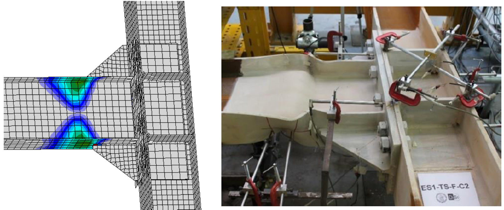
Fig. 12.2.3 Validarea modului de cedare CBFEM pe îmbinările cu placă de capăt extinsă și vută E1-TS-F-C2 (Tartaglia și D'Aniello, 2017)

Fig.12.2.4 Validarea rezistenței CBFEM pe experimente din proiectul EQUALJOINTS

Fig. 12.2.5 Validarea capacității de rotație CBFEM pe experimente din proiectul EQUALJOINTS

12.2.2 Verificare

Modelul CBFEM a fost verificat față de metoda componentelor (CM) conform Cap. 6 din EN 1993-1-8:2006. Selecția rezultatelor este prezentată în Tab. 12.2.1 și Fig. 12.2.6. Rezultatele evidențiază pierderea preciziei metodei CM pentru îmbinările de dimensiuni mai mari, unde ipoteza aproximativă privind brațul de pârghie influențează acuratețea.

Tab. 12.2.1 Verificarea CBFEM față de CM

Tipologie	Rezistență
#	CM	CBFEM	CBFEM/CM	Componentă decisivă
	MR [kNm]	MR [kNm]	[%]
		Îmbinare cu vută
EH2-TS35-M	901,2	889	1	Placă de capăt la încovoiere
EH2-TS45-M	959,3	875	10	Placă de capăt la încovoiere
4.2	876,1	1 016	−16	Talpa stâlpului la încovoiere
264	545,4	573	−5	Talpa stâlpului la încovoiere
267	1 998,9	2 100	−5	Placă de capăt la încovoiere
		Îmbinare extinsă rigidizată
ES1-TS-F-M	547,5	533	3	Talpa stâlpului la încovoiere
ES3-TS-F-M	1389	1 920	−27	Talpa stâlpului la încovoiere
		Îmbinare extinsă nerigidizată
E1-TB-E-M	347,8	389	−11	Placă de capăt la încovoiere
E2-TB-E-M	577,0	681	−15	Placă de capăt la încovoiere

Fig. 12.2.6 Verificarea rezistenței CBFEM față de CM

Trei îmbinări cu vută unilaterală sunt descrise mai detaliat în (Landolfo et al. 2017) și (aplicația Equaljoints). Îmbinările sunt încărcate atât cu momente încovoietoare pozitive, cât și negative și cu forța tăietoare corespunzătoare. Inimile stâlpilor sunt consolidate cu dubluri, astfel încât componentele decisive sunt T-stub-urile fie ale plăcii de capăt, fie ale tălpii stâlpului. Axele de rotație sunt presupuse la centrul tălpii superioare a grinzii pentru momentul încovoietor pozitiv și la mijlocul vutei pentru momentul încovoietor negativ. Poziția articulației plastice este presupusă la fața plăcii de rigidizare de la capătul vutei. Momentul încovoietor la fața stâlpului utilizat pentru verificarea îmbinării este majorat cu forța tăietoare corespunzătoare; a se vedea Fig. 12.2.7.

Fig. 12.2.7 Poziția articulației plastice, diagrama momentului încovoietor în îmbinarea cu vută

Tab. 12.2.2 Rezistența componentelor prin CM pentru îmbinările cu vută

Rezistența componentelor prin CM	#4.2 (IPE450 la HEB340)	#264 (IPE360 la HEB280)	#267 (IPE600  la HEB500)
Moment la articulația plastică [kNm]	906	543	1869
Forță tăietoare [kN]	295	148	561
Moment la fața stâlpului [kNm]	981	573	2105
Rezistența vutei [kNm]	956	582	1903
Forța tăietoare care acționează pe inima stâlpului [kN]	1581	1035	2447
Rezistența inimii stâlpului la forfecare [kN]	1632	1203	2774
T-stub - placă de capăt - moment negativ [kNm]	1019	573	1999
T-stub - placă de capăt - moment pozitiv [kNm]	1081	697	2318
T-stub - talpa stâlpului - moment negativ [kNm]	876	545	2015
T-stub - talpa stâlpului - moment pozitiv [kNm]	929	580	2107

Factorul de ecruisare a fost ales 1,2 conform recomandărilor din EN 1993-1-8:2006 și raportul final al proiectului Equaljoints (EN 1998-1:2005 sugerează valoarea 1,1). Factorul de suprarezistență a fost presupus 1,25 (Landolfo et al. 2017). Tot oțelul a fost de clasa S355. Rezistențele componentelor individuale sunt rezumate în Tab. 12.2.2. Verificările marcate cu bold nu sunt satisfăcute. De remarcat că rezistența vutei reprezintă rezistența plastică a secțiunii grinzii cu vuta la placa de capăt. Rezistența grinzii este presupusă majorată cu factorul de suprarezistență la locul articulației plastice, dar nu și la placa de capăt. Dacă factorul de suprarezistență ar fi aplicat și la placa de capăt, această rezistență ar fi mai mare. Prin urmare, următoarea rezistență cea mai mică, T-stub – placă de capăt, a fost considerată ca guvernând rezistența îmbinării nr. 267. Niciuna dintre îmbinările investigate nu satisface cerința pentru îmbinare cu rezistență totală. Cu toate acestea, rezistența este foarte apropiată, iar îmbinările sunt cu rezistență egală. Panoul inimii stâlpului este puternic în toate cazurile.

Modul de cedare determinant conform CBFEM este cedarea șuruburilor cu curgerea plăcilor, în principal a plăcii de capăt, a tălpii stâlpului și a vutei. Conform CBFEM, îmbinările nr. 4.2 și nr. 264 sunt cu rezistență totală, iar îmbinarea nr. 267 este cu rezistență egală. Panourile inimii stâlpului sunt puternice în toate cazurile.

Fig. 12.2.8 Deformațiile la rezistență pentru a) întreaga îmbinare, b) numai macro-componenta îmbinare cu placă de capăt cu șuruburi, c) numai macro-componenta panou de inimă al stâlpului la forfecare cu dubluri de inimă, d) numai macro-componenta grindă

12.2.3 Îmbinări cu placă de capăt extinsă nerigidizată

Pentru studiul de sensibilitate, a fost selectată o îmbinare precalificată cu placă de capăt extinsă nerigidizată. Grinda IPE 450 este conectată la stâlpul HEB 300 printr-o placă de capăt extinsă cu grosimea de 25 mm cu douăsprezece șuruburi M30 10.9, cu și fără dublură de inimă de 10 mm grosime. Oțelul de clasa S 355 a fost utilizat pentru toate plăcile. Pentru a determina contribuția fiecărei macro-componente în mod separat, diagrama de material a macro-componentei selectate a fost elastoplastică, în timp ce restul îmbinării a avut doar diagramă de material elastică. Deformațiile la rezistența întregii îmbinări, a panoului inimii stâlpului la forfecare numai cu dubluri de inimă și a îmbinării cu placă de capăt cu șuruburi sunt comparate cu macro-componenta grindă în Fig. 12.2.8. Influența fiecărei macro-componente asupra comportamentului îmbinării este prezentată în Fig. 12.2.9, unde panoul inimii stâlpului cu și fără dubluri de inimă este ilustrat. Comportamentul îmbinării evidențiază o rezistență mai mare a macro-componentei îmbinare.

Fig. 12.2.9 Influența macro-componentelor, panoul inimii stâlpului cu dubluri la forfecare,
îmbinarea cu placă de capăt cu șuruburi și grinda asupra comportamentului întregii îmbinări

12.2.4 Localizarea centrului de compresiune

Pentru îmbinările cu placă de capăt, EN 1993-1-8:2006 specifică faptul că centrul de compresiune este situat la mijlocul grosimii tălpii grinzii sau la vârful vutei în cazul îmbinărilor cu vută. Rezultatele experimentale și numerice au arătat că localizarea centrului de compresiune depinde atât de tipul îmbinării, cât și de cererea de rotație, datorită formării modurilor plastice cu angajare diferită a fiecărei componente a îmbinării (Landolfo et al. 2017). Conform procedurii de proiectare CM propuse și pe baza rezultatelor atât experimentale, cât și numerice, se estimează un contact în apropierea centroidului secțiunii formate din talpa grinzii și nervurile de rigidizare, pentru îmbinările cu placă de capăt rigidizată, sau la aproximativ 0,5 din înălțimea vutei în cazul îmbinărilor cu vută. Această ipoteză aproximativă este precizată de procedura CBFEM, care furnizează valori corecte în timpul încărcării și al curgerii inițiale a părților îmbinării.

Rezultatele prezentate demonstrează acuratețea bună a CBFEM verificat față de ROFEM și validat pe experimentele EQUALJOINTS și CM. Aceasta oferă posibilitatea de a considera comportamentul macro-componentelor în mod separat și poziția axelor neutre cu precizie în funcție de încărcare/plastificare.

12.3 Îmbinare cu secțiune de grindă redusă sudată

O îmbinare precalificată cu secțiune de grindă redusă sudată conform ANSI/AISC 358-16 a fost selectată pentru acest studiu. Grinda IPE 450 este conectată la stâlpul HEB 300 prin suduri cap la cap la tălpi și o placă de inimă de 12 mm grosime cu trei șuruburi pretensionate M30 10.9, cu și fără dublură de inimă de 10 mm grosime; a se vedea Fig. 12.3.1. Tot oțelul utilizat este de clasa S355.

Deformațiile la rezistența ultimă a întregii îmbinări și ale macro-componentei panou de inimă al stâlpului la forfecare numai cu dubluri de inimă sunt prezentate în Fig. 12.3.2. Influența fiecărei macro-componente asupra comportamentului îmbinării este prezentată în Fig. 12.3.3, unde panoul inimii stâlpului cu și fără dubluri de inimă este ilustrat. Îmbinarea arată că rezistențele macro-componentelor sunt bine optimizate.

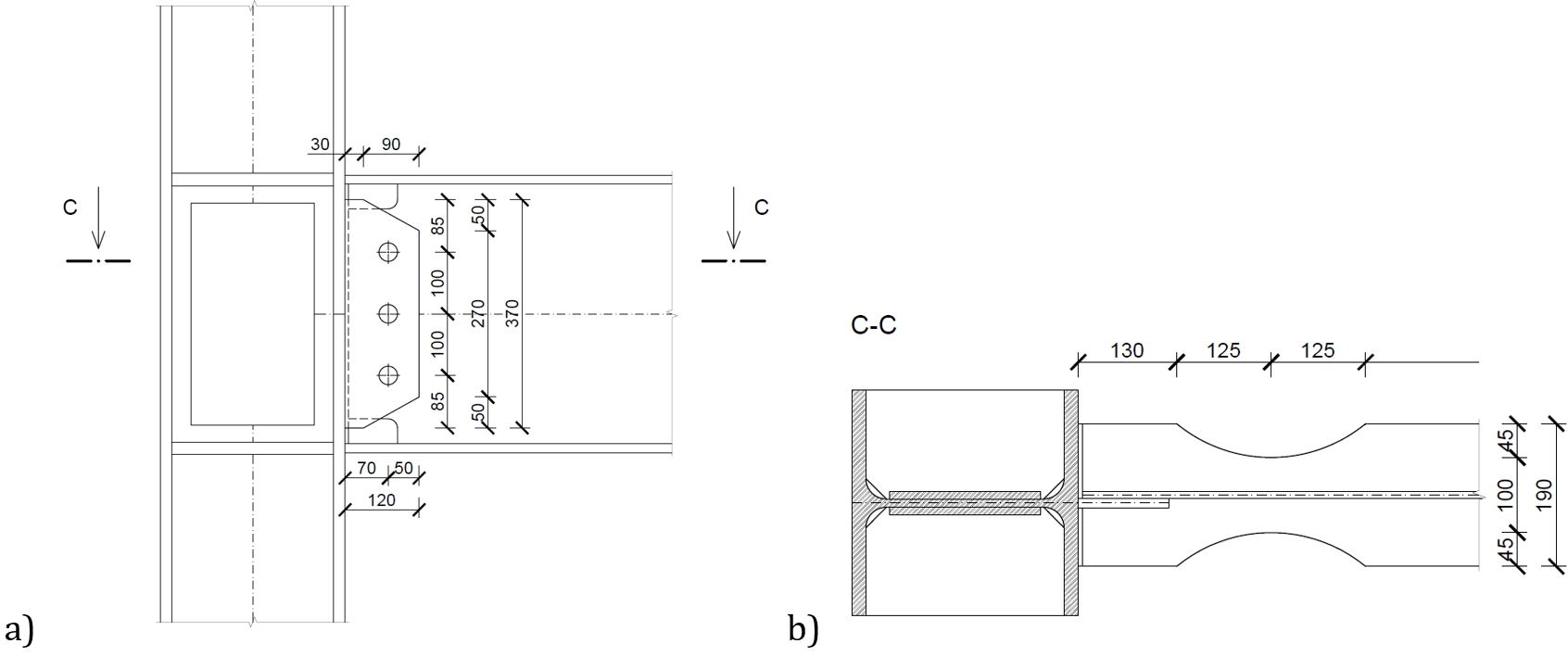
Fig. 12.3.1 Îmbinare cu secțiune de grindă redusă, a) grindă cu secțiune redusă, b) panoul inimii stâlpului cu dubluri la forfecare, îmbinarea cu placă de capăt cu șuruburi,

Fig. 12.3.2 Deformațiile la rezistență pentru a) întreaga îmbinare și b) numai macro-componenta panou de inimă al stâlpului cu dubluri la forfecare 

Fig. 12.3.3 Influența macro-componentelor asupra comportamentului întregii îmbinări pe diagrama M-φ

Referințe

EN 1993-1-8, Eurocode 3, Proiectarea structurilor de oțel – Partea 1-8: Proiectarea îmbinărilor, CEN, Bruxelles, 2005.

Jones S.L., Fry GT., Engelhardt M.D. Evaluare experimentală a îmbinărilor cu moment rezistent și secțiune de grindă redusă solicitate ciclic. Journal of Structural Engineering. 128 (4), 441–451, 2002.

Landolfo R. et al. Proiectarea structurilor de oțel pentru clădiri în zone seismice, Manual de proiectare ECCS Eurocode. Wiley, 2017.

Stratan A., Maris C, Dubina D, și Neagu C. Precalificarea experimentală a îmbinărilor grindă-stâlp cu șuruburi și placă de capăt extinsă cu vute. ce/papers, 1(2–3), 414–423, 2017.

Tartaglia R, D'Aniello M. Comportamentul neliniar al îmbinărilor grindă-stâlp cu șuruburi și placă de capăt extinsă rigidizată supuse eliminării stâlpului. The Open Civil Engineering Journal Vol 11, Issue Suppl-1, 369–383, 2017.

Zhang X., Ricles J.M. Evaluare experimentală a îmbinărilor cu secțiune de grindă redusă la stâlpi cu înălțime mare. Journal of Structural Engineering. 132 (3), 346-357, 2006.