Fatigue analysis according to EN 1993-1-9
This article shows how to use nominal stresses provided by IDEA Connection to perform full fatigue analysis according to EN 1993-1-9.
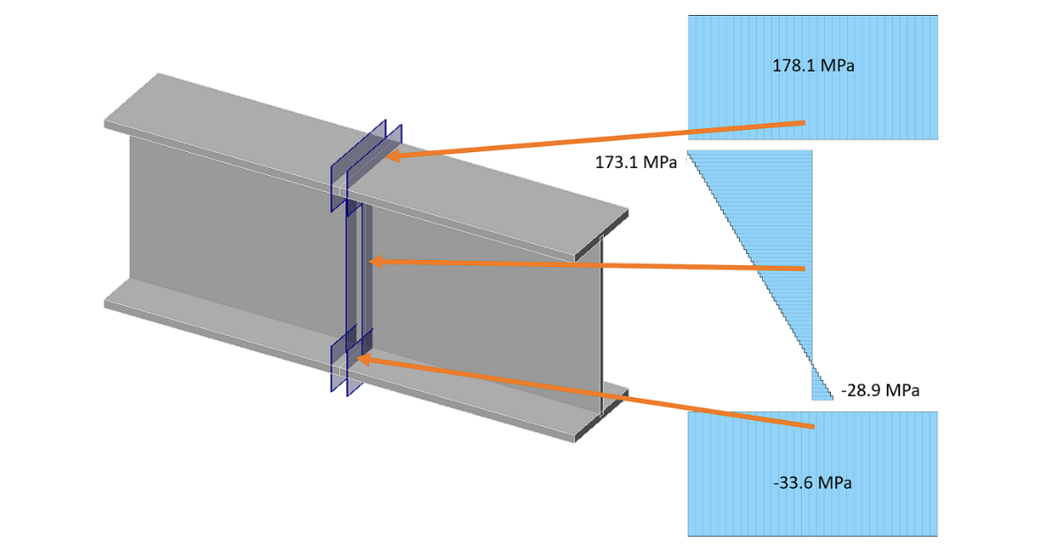
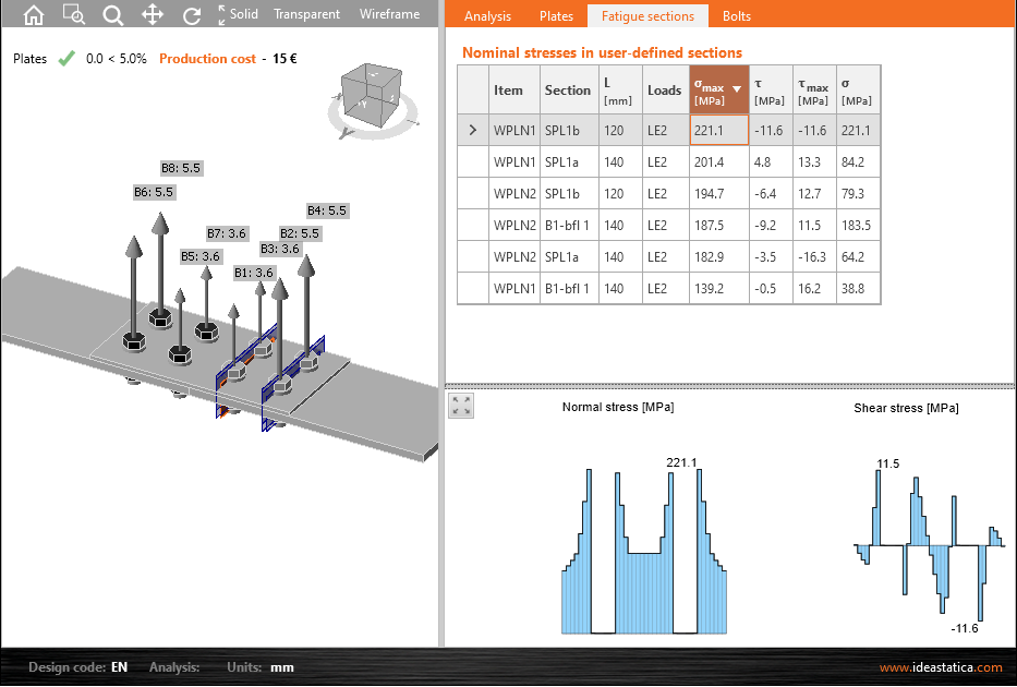
IDEA Connection provides nominal stresses in:
- user-defined sections
- sections near welds
- bolts and anchors
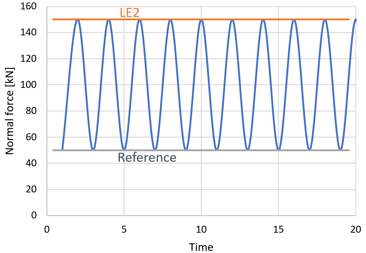
The provided stresses are the stress range between the load effect and the reference load effect. The stress range is not modified in any way, e.g. in terms of the below-shown figure, which allows decreasing the stress range if the stress changes from tension to compression.
These stresses include some stress concentration factors, e.g. concentration of stresses near bolt holes.
Other factors, e.g. partial factor for equivalent constant amplitude stress ranges \(\gamma_{Ff}\) according to EN 1991 or k1 factors for hollow section joints due to neglected bending moments in truss model still have to be included.
IDEA Connection provides \(\sigma_{max}\) and \(\tau_{max}\) to be used to obtain \(\Delta \sigma\) and \(\Delta \tau\).
\[ \Delta \sigma = \gamma_{Ff} \cdot k_x \cdot \sigma_{max}\]
\[ \Delta \tau = \gamma_{Ff} \cdot k_x \cdot \sigma_{max}\]
where:
- \(\gamma_{Ff}\) – partial factor for equivalent constant amplitude stress ranges
- \(k_x\) – any factors not included in the analysis, e.g. \(k_1\) from Table 4.1 or 4.2
- \(\sigma_{max}\) – IDEA Connection output of normal stress
- \(\tau_{max}\) – IDEA Connection output of shear stress
According to Chapter 8, Equation (8.1), following stress limitations must be satisfied:
\[\Delta \sigma \le 1.5 f_y\]
\[\Delta \tau \le 1.5 f_y / \sqrt{3}\]
where \(f_y\) is steel yield strength.
The detail has to be categorized according to Tables 8.1–8.10 and all relevant factors must be taken into account, e.g. the factor for size effects. The detail category (reduced by e.g. size effect factor) provides the fatigue strength at 2 million cycles, \(\Delta \sigma_c\) and \(\Delta \tau_c\). The values of \(\Delta \sigma_c\) and \(\Delta \tau_c\) should be reduced by partial factor for fatigue strength, \(\gamma_{Mf}\).
Table 3.1 from EN 1993-1-9 with values of \(\gamma_{Mf}\):
| Assessment method | Consequence of failure | |
| Low consequence | High consequence | |
| Damage tolerant | 1 | 1.15 |
| Safe life | 1.15 | 1.35 |
The limits of S-N (stress-life) curve are determined according to Chapter 7.1:
\[\Delta \sigma_D = \left ( \frac{2}{5} \right )^{1/3} \Delta \sigma_c \]
\[\Delta \sigma_L = \left ( \frac{5}{100} \right )^{1/5} \Delta \sigma_D \]
\[\Delta \tau_L = \left ( \frac{2}{100} \right )^{1/5} \Delta \tau_c \]
According to Chapter A.5, cycles to failure should be determined. Number of cycles, \(n_{Ei}\), associated with stress range \(\gamma_{Ff} \Delta \sigma_i\), is an input from the user. \(N_{Ri}\) is calculated according to Chapter 7.
Normal stresses for \(\Delta \sigma \ge \Delta \sigma_D\):
\[N_R = \frac{\Delta \sigma_c^m \cdot 2\cdot 10^6}{\Delta \sigma^m}\]
where:
- m = 3 – slope of fatigue strength curve
Normal stresses for \(\Delta \sigma \ge \Delta \sigma_L\):
\[N_R = \frac{\Delta \sigma_D^m \cdot 5\cdot 10^6}{\Delta \sigma^m} \]
where:
- m = 5 – slope of fatigue strength curve
The normal stresses below cut-off limit \(\Delta \sigma_L\) do not participate to fatigue damage.
Shear stresses for \(\Delta \tau_E \le \Delta \tau_L\):
\[N_R = \frac{\Delta \tau_c^m \cdot 2\cdot 10^6}{\Delta \tau^m} \]
where:
- m = 5 – slope of fatigue strength curve
The shear stresses below the cut-off limit \(\Delta \tau_L\) do not participate in fatigue damage.
The damage is calculated according to Palmgren-Miner rule (Figure A.1) in Equations (A.1) and (A.2) separately for normal and shear stress:
\[D_d = \Sigma_i^n \frac{n_{Ei}}{N_{Ri}} \le 1.0\]
The normal stress and shear stress should be combined by Equation (8.3), unless otherwise stated in Tables 8.8 and 8.9.
\[D_{d \sigma}^3 + D_{d \tau}^5 \le 1.0 \]
Example
Inputs for calculation: The user sets a reference load effect and three fatigue load effects. The outputs from IDEA Connection are the maximum normal stress and the corresponding shear stress. The steel grade is S355.
| Load effect | Number of cycles | Maximum normal stress | Corresponding shear stress |
| nE | Δσmax [MPa] | Δτ [MPa] | |
| LE2 | 1 500 000 | 60 | 60 |
| LE3 | 3 000 000 | 50 | 40 |
| LE4 | 10 000 000 | 20 | 10 |
Partial safety factors are determined from EN 1991 and EN 1993-1-9:
\[ \gamma_{Ff} = 1.0 \]
\[ \gamma_{Mf} = 1.15 \]
Stress limitations are checked:
\[\Delta \sigma \le 1.5 f_y\]
\[ 60 \, \textrm{MPa} \le 1.5 \cdot 355 = 532 \, \textrm{MPa}\]
\[\Delta \tau \le 1.5 f_y / \sqrt{3} \]
\[60 \, \textrm{MPa} \le 1.5 \cdot 355 / \sqrt{3} = 307 \, \textrm{MPa} \]
From Tables 8.1–8.10, values of \(\Delta \sigma_c = 90\,\textrm{MPa}\) and \(\Delta \tau_c = 70\,\textrm{MPa}\) are determined. These values are reduced by reduced by partial factor for fatigue strength, \(\gamma_{Mf} = 1.15\) to \(\Delta \sigma_c = 78.3\,\textrm{MPa}\) and \(\Delta \tau_c = 60.9\,\textrm{MPa}\).
The limits of S-N curve are determined:
\[\Delta \sigma_D = \left ( \frac{2}{5} \right )^{1/3} \Delta \sigma_c = \left ( \frac{2}{5} \right )^{1/3} 78.3 = 57.7\,\textrm{MPa}\]
\[\Delta \sigma_L = \left ( \frac{5}{100} \right )^{1/5} \Delta \sigma_D = \left ( \frac{5}{100} \right )^{1/5} 57.7 = 31.7 \,\textrm{MPa}\]
\[\Delta \tau_L = \left ( \frac{2}{100} \right )^{1/5} \Delta \tau_c = \left ( \frac{2}{100} \right )^{1/5} 60.9 = 27.8\,\textrm{MPa} \]
\(\Delta \sigma\) is determined by multiplying \(\Delta \sigma_{max}\) by partial factor for equivalent constant amplitude stress ranges \(\gamma_{Ff} = 1.0\). In this example, no other factor kx is necessary.
Number of cycles to failure, \(N_R\) is calculated for each load case and normal and shear stress according to the above-mentioned formulas, e.g. for normal stress in LE2:
\[N_R = \frac{\Delta \sigma_c^m \cdot 2\cdot 10^6}{\Delta \sigma^m} = \frac{78.3^3 \cdot 2\cdot 10^6}{60^3} = 4 \,438\, 234 \, \textrm{cycles}\]
| Load effect | Number of cycles | Maximum normal stress | Corresponding shear stress | Number of cycles to failure | Number of cycles to failure | ||
| nE | Δσmax [MPa] | Δτ [MPa] | Δσ [MPa] | NR | Δτ [MPa] | NR | |
| LE2 | 1 500 000 | 60 | 60 | 60 | 4 438 235 | 60 | 2 149 190 |
| LE3 | 3 000 000 | 50 | 40 | 50 | 10 200 230 | 40 | 16 320 409 |
| LE4 | 10 000 000 | 20 | 10 | 20 | infinity | 10 | infinity |
Using Palmgren-Miner rule, the accumulated damage is calculated for all load effects.
For normal stresses:
\[D_{d \sigma} = \Sigma_i^n \frac{n_{Ei}}{N_{Ri}} = \frac{1\, 500\, 000}{4\, 438\, 235} + \frac{3\,000\,000}{10\,200\,230} = 0.632 \le 1.0\]
For shear stresses:
\[D_{d \tau} = \Sigma_i^n \frac{n_{Ei}}{N_{Ri}} = \frac{1\, 500\, 000}{2\, 149\, 190} + \frac{3\,000\,000}{16\,320\,409} = 0.882 \le 1.0\]
Finally, the interaction between normal and shear stress is checked:
\[ D_{d \sigma} ^3 + D_{d \tau} ^5 \le 1.0\]
\[ 0.632 ^3 + 0.882 ^5 = 0.786 \le 1.0\]
The fatigue resistance of the investigated detail is sufficient.
Verifications
Before releasing the Fatigue analysis tool, several experimental verifications have been performed:
Fatigue life by nominal stress method
Fatigue analysis – Butt welds of I section