Tutorial

Erste Schritte mit der API – Komponenten in einer Verbindung optimieren 04

Stahl

Connection

IDEA Open Model (API)

Overall check

Parametric design

Stress/strain

Dieser Artikel ist auch verfügbar in:

Mit KI aus dem Englischen übersetzt

In diesem Tutorial erfahren Sie, wie Sie mithilfe von Parametern einige Komponenten (Schweißnähte, Schrauben) in einer Verbindung optimieren können.

Erste Schritte

Wir empfehlen, das Tutorial Erste Schritte mit der API – Grundlagen 01 durchzuarbeiten, das Ihnen die API und die Einrichtung der Umgebung erklärt.

Connection-Datei

Dieses Beispiel basiert auf Dateien, die im Tutorial Erste Schritte mit der API – Vorlage importieren und Berechnung ausführen 03 erstellt wurden.

Bitte laden Sie die Datei tutorial 03 with template-new.ideaCon herunter.

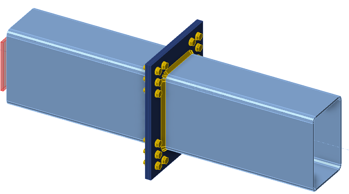
Wir möchten die Komponenten der Verbindung (Schweißnähte, Durchmesser und Anzahl der Schrauben) optimieren. Das Ergebnis der Optimierung sind die Kosten der Verbindung, die übersichtlich in einem Diagramm dargestellt werden.

Python-Client

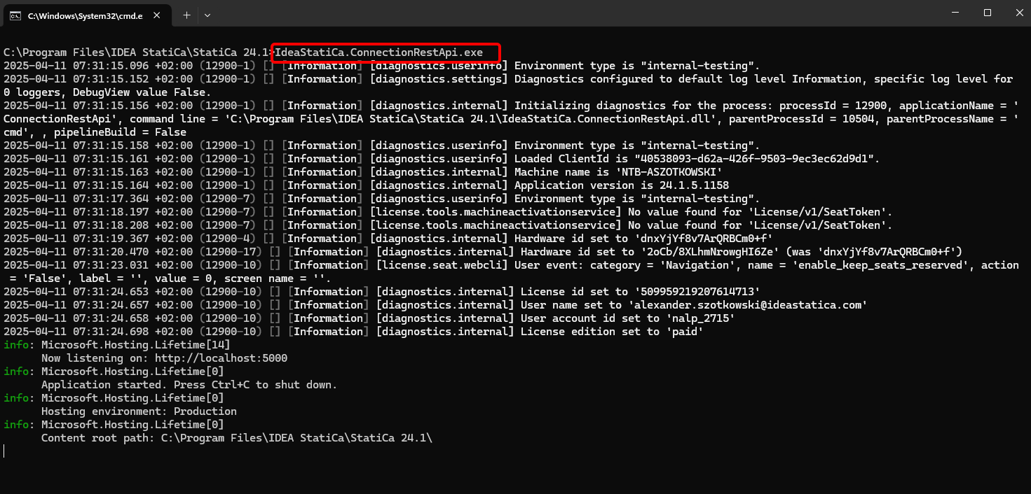
Führen Sie "IdeaStatiCa.ConnectionRestApi.exe" in CMD im entsprechenden IDEA StatiCa-Ordner aus und öffnen Sie das IDE-Werkzeug Ihrer Wahl.

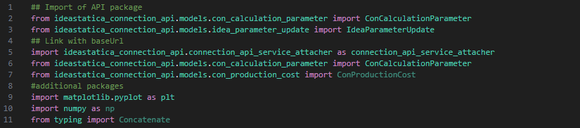
Erstellen Sie eine neue Datei und importieren Sie die Pakete, die die Verwendung der Berechnung und die Verknüpfung mit der localhost-URL ermöglichen.

Quellcode:

## Import of API package
from ideastatica_connection_api.models.con_calculation_parameter import ConCalculationParameterfrom ideastatica_connection_api.models.idea_parameter_update import IdeaParameterUpdate

## Link with baseUrl
import ideastatica_connection_api.connection_api_service_attacher as connection_api_service_attacher
from ideastatica_connection_api.models.con_calculation_parameter import ConCalculationParameterfrom ideastatica_connection_api.models.con_production_cost import ConProductionCost

#additional packages
import matplotlib.pyplot as plt
import numpy as np
from typing import Concatenate

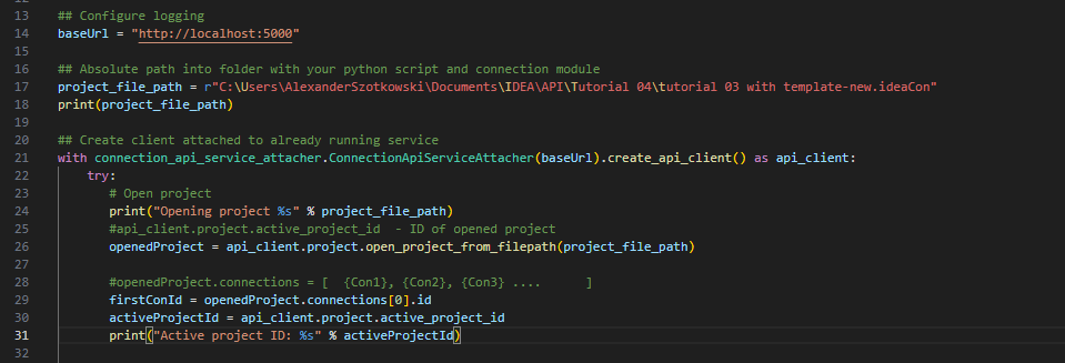
Konfigurieren Sie das Logging über die Variable "baseUrl", die Ihren localhost aufruft. Im zweiten Schritt verknüpfen Sie den absoluten Pfad Ihrer IDEA StatiCa Connection-Datei.

## Configure logging
baseUrl = "http://localhost:5000"

## Absolute path into folder with your python script and connection module
project_file_path = r"C:\Users\AlexanderSzotkowski\Documents\IDEA\API\Tutorial 04\tutorial 03 with template -new.ideaCon"
print(project_file_path)

Verbinden Sie den Client mit einem bereits laufenden Dienst. Verwenden Sie den try/except-Block – da der try-Block einen Fehler auslöst, wird der except-Block ausgeführt. In der ersten Phase muss das Projekt geöffnet und die Projekt-ID Ihres Projekts ermittelt werden, die für jedes IDEA StatiCa-Projekt eindeutig ist. Anschließend wählen wir die erste in unserer Datei gespeicherte Verbindung aus.

# Create a client attached to an already running service
with connection_api_service_attacher.ConnectionApiServiceAttacher(baseUrl).create_api_client() as api_client:
try:
# Open project
print("Opening project %s" % project_file_path)
#api_client.project.active_project_id - ID of opened project
openedProject = api_client.project.open_project_from_filepath(project_file_path)

#openedProject.connections = [ {Con1}, {Con2}, {Con3} .... ]
firstConId = openedProject.connections[0].id
activeProjectId = api_client.project.active_project_id
print("Active project ID: %s" % activeProjectId)

Alle benötigten Parameter aus der ideaCon-Datei abrufen (Anzahl der Schrauben, Durchmesser, Schweißnahtgröße, Schraubengarnitur)

#get parameters from ideaCon file
include_hidden = True
parameters = api_client.parameter.get_parameters(activeProjectId, firstConId, include_hidden=include_hidden)
#get default values from the ideaCon file
#Diameter of the bolt
boltParameter = parameters[3]
#print('bolt ',boltParameter.value)
#Number of bolt rows
rowParameter = parameters[11]
#print('row ',rowParameter.value)
#Weld size
weldParameter = parameters[28]
#print('weld ',weldParameter.value)
#Bolt assembly
boltAssemblyParameter = parameters[29]
#print('bolt assembly ',boltAssemblyParameter.value)

Wir möchten Ergebnisse nur dann erhalten, wenn die Berechnung für alle Teile (Bleche, Schweißnähte, Schrauben) zu 100 % positiv ist. Daher müssen wir Stop at the limit strain auf True setzen. Die Ergebnisse werden in einer Liste namens matrix gespeichert, die wir anschließend zur Darstellung eines Diagramms verwenden.

#setup
updateSettings = api_client.settings.get_settings(api_client.project.active_project_id)

from typing import Dict
updateSettings: Dict [str, object] = {
"calculationCommon/Analysis/AnalysisGeneral/Shared/StopAtLimitStrain@01" : True,
"calculationCommon/Checks/Shared/LimitPlasticStrain@01" : 0.05
}
api_client.settings.update_settings(api_client.project.active_project_id, updateSettings)

#Final results database
matrix = []

Nun starten wir einen Zyklus, bei dem die Schweißnähte (von t = 8 auf 5 mm), der Schraubendurchmesser (von M16 auf M12) und die Anzahl der Reihen (von 3 auf 1) variiert werden. Die Werte 8, M16 und 3 stammen aus der ideaCon-Datei. Die laufenden Ergebnisse werden auf dem Bildschirm ausgegeben und der Ergebnisliste hinzugefügt.

#cycling through welds with given rows and bolts
for row in range(rowParameter.value,1, -1):
#print ('Number of bolt rows is', row)
for bolt in range(int(1000*boltParameter.value), 12,-2):

for weld in range(int(1000*weldParameter.value), 5,-1):

par_row = IdeaParameterUpdate() # Create a new instance
par_row.key = rowParameter.key
par_row.expression = str(row)

par_bolt = IdeaParameterUpdate() # Create a new instance
par_bolt.key = boltParameter.key
par_bolt.expression = str(bolt/1000) # Decrement the expression

par_boltAssembly = IdeaParameterUpdate() # Create a new instance
par_boltAssembly.key = boltAssemblyParameter.key
par_boltAssembly.expression = str('M'+ str(bolt) + ' 8.8')

par_weld = IdeaParameterUpdate() # Create a new instance
par_weld.key = weldParameter.key
par_weld.expression = str(weld/1000) # Decrement the expression

updateResponse = api_client.parameter.update(activeProjectId, firstConId, [par_row, par_bolt, par_boltAssembly, par_weld] )
updateResponse.set_to_model

# Check if the parameters were updated successfully
if updateResponse.set_to_model == False:
print('Parameters failed: %s' % ', '.join(updateResponse.failed_validations))

#set the type of analysis
ConCalculationParameter.analysis_type = "stress_strain"

conParameter = ConCalculationParameter()
conParameter.connection_ids = [ firstConId ]
summary = api_client.calculation.calculate(activeProjectId, conParameter.connection_ids)

# Get results after calculation, store it in separate file and print the actual results
results = api_client.calculation.get_results(activeProjectId, conParameter.connection_ids)
CheckResSummary = results[0].check_res_summary
costs = api_client.connection.get_production_cost(api_client.project.active_project_id, firstConId)

api_client.project.download_project(activeProjectId, r'C:\Users\AlexanderSzotkowski\Documents\IDEA\API\Tutorial 04\tutorial 03 with template-updated.ideaCon')

if CheckResSummary[0].check_status == False:
break

if CheckResSummary[0].check_status == True:
print (row,'rows of', bolt, 'bolts', 'and weld size ',par_weld.expression,' results are OK. Costs: ', costs.total_estimated_cost)
values= [row, bolt,par_weld.expression,costs.total_estimated_cost]
#print(values)
matrix.append(values)

else:
print ('Iteration %i failed' % weld)

else:
print ('Iteration %i for weld failed' % weld)

else:
print ('Iteration %i for bolts failed' % bolt)

else:
print ('Iteration %i for rows failed' % row)

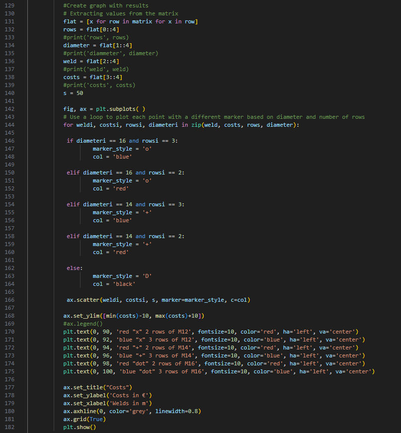
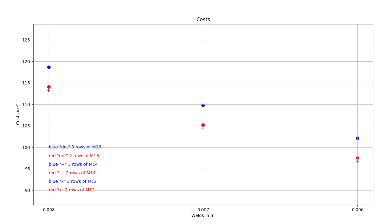
Der letzte Teil befasst sich mit der Erstellung eines Diagramms mit unseren Ergebnissen.

#Create graph with results
# Extracting values from the matrix
flat = [x for row in matrix for x in row]
rows = flat[0::4]
#print('rows', rows)
diameter = flat[1::4]
#print('diammeter', diameter)
weld = flat[2::4]
#print('weld', weld)
costs = flat[3::4]
#print('costs', costs)
s = 50

fig, ax = plt.subplots( )
# Use a loop to plot each point with a different marker based on diameter and number of rows
for weldi, costsi, rowsi, diameteri in zip(weld, costs, rows, diameter):

if diameteri == 16 and rowsi == 3:
marker_style = 'o'
col = 'blue'

elif diameteri == 16 and rowsi == 2:
marker_style = 'o'
col = 'red'

elif diameteri == 14 and rowsi == 3:
marker_style = '+'
col = 'blue'

elif diameteri == 14 and rowsi == 2:
marker_style = '+'
col = 'red'

else:
marker_style = 'D'
col = 'black'

ax.scatter(weldi, costsi, s, marker=marker_style, c=col)

ax.set_ylim([min(costs)-10, max(costs)+10])

#ax.legend()
plt.text(0, 90, 'red "x" 2 rows of M12', fontsize=10, color='red', ha='left', va='center')
plt.text(0, 92, 'blue "x" 3 rows of M12', fontsize=10, color='blue', ha='left', va='center')
plt.text(0, 94, 'red "+" 2 rows of M14', fontsize=10, color='red', ha='left', va='center')
plt.text(0, 96, 'blue "+" 3 rows of M14', fontsize=10, color='blue', ha='left', va='center')
plt.text(0, 98, 'red "dot" 2 rows of M16', fontsize=10, color='red', ha='left', va='center')
plt.text(0, 100, 'blue "dot" 3 rows of M16', fontsize=10, color='blue', ha='left', va='center')

ax.set_title("Costs")
ax.set_ylabel('Costs in €')
ax.set_xlabel('Welds in m')
ax.axhline(0, color='grey', linewidth=0.8)
ax.grid(True)
plt.show()

Wie Sie sehen können, ist in diesem speziellen Fall die wirtschaftlichste Verbindung diejenige mit einer 6 mm Schweißnaht und drei Reihen von M14-Schrauben.