The objective
The objective of this article is the verification of the LBA (linear bifurcation analysis) module of the IDEA Member application. The resulting critical loads from IDEA Member are compared to Euler’s critical loads for columns in compression.
Model description
A total of 24 individual cases were analyzed to verify the LBA module. All of them share the same cross-section HEB 200 and the same steel grade S 355. Four different boundary conditions were investigated (FF; PP; FP; FF), each with varying values of columns relative slenderness (0.5; 1.0; 1.5). Buckling in direction of both principal axes is verified.
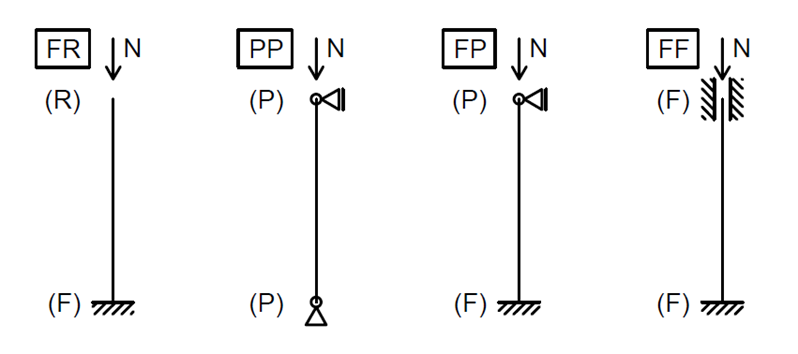
Fig. 1: Various boundary conditions used for verification
All cases are designated in the following manner: “FR_0.5_Y”, where “FR” indicates boundary conditions, “0.5” the relative slenderness and “Y” the buckling axis.
Cross-section description
There is a slight difference in characteristics of a rolled HEB 200 cross-section and its shell representation in IDEA Member. Its influence on the critical load is later shown to be under 2 % for strong axis buckling and under 1 % for weak axis buckling.
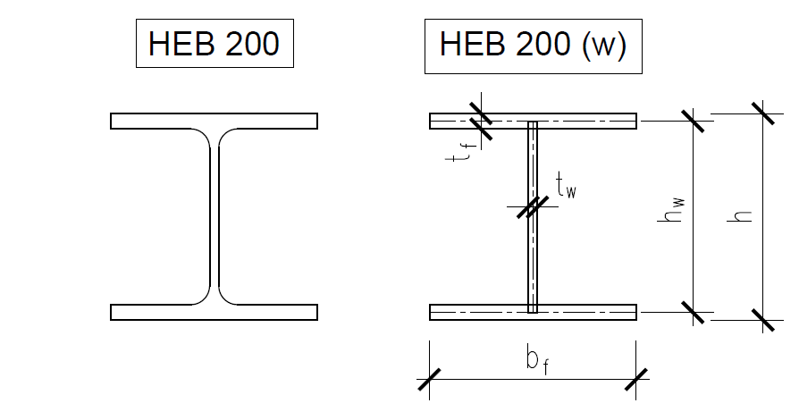
Fig. 2: Rolled cross-section and its shell representation
Analytical solution
The following formula is used to calculate the Euler’s critical load for strong and weak axis buckling:
\[ N_{cr,y(z)} = \frac{\pi^2EI_{y(z)}}{L_{cr,y(z)}^2} \]
The buckling length for individual cases relative to the system length is:
FR (Fixed – Free) \(L_{cr,y(z)} = 2.0 \cdot L \)
PP (Pinned – Pinned) \(L_{cr,y(z)} = 1.0 \cdot L \)
FP (Fixed – Pinned) \(L_{cr,y(z)} = 0.7 \cdot L \)
FF (Fixed – Fixed) \(L_{cr,y(z)} = 0.5 \cdot L \)
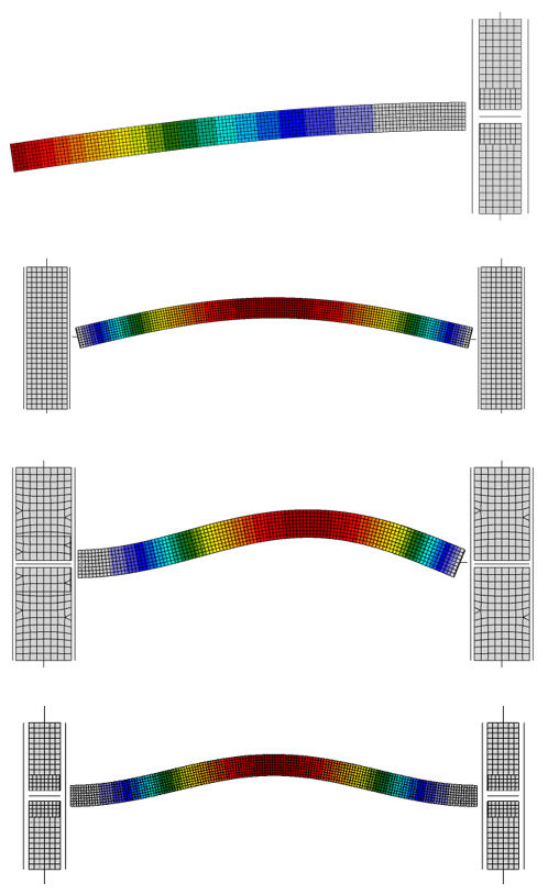
Fig. 3: Weak axis buckling modes for the four different boundary conditions
Results
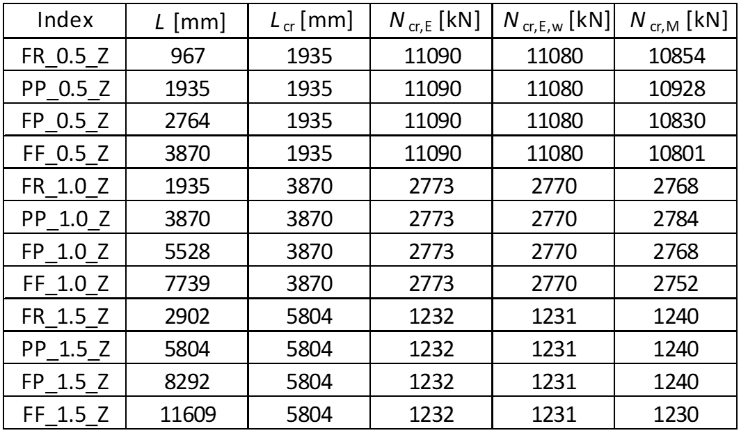
The critical load from IDEA Member (M) is compared to an analytical value for a rolled cross-section (E) and for its representation without the web-flange radii (Ew) as well.
Strong axis buckling
The results for strong axis buckling are summarized in the table below.
Tab. 1: Resulting critical loads – axis y-y
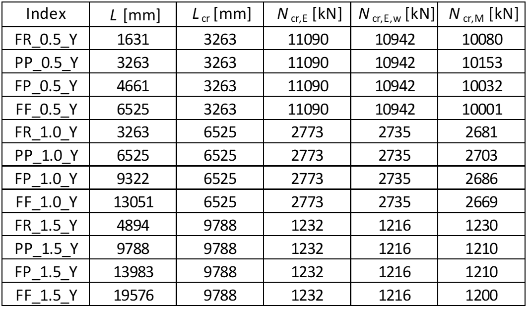
The results of LBA are slightly conservative (< 10 %) for columns with low relative slenderness. For higher relative slenderness, the critical loads are conservative and very close to the expected analytical value (< 4 %).
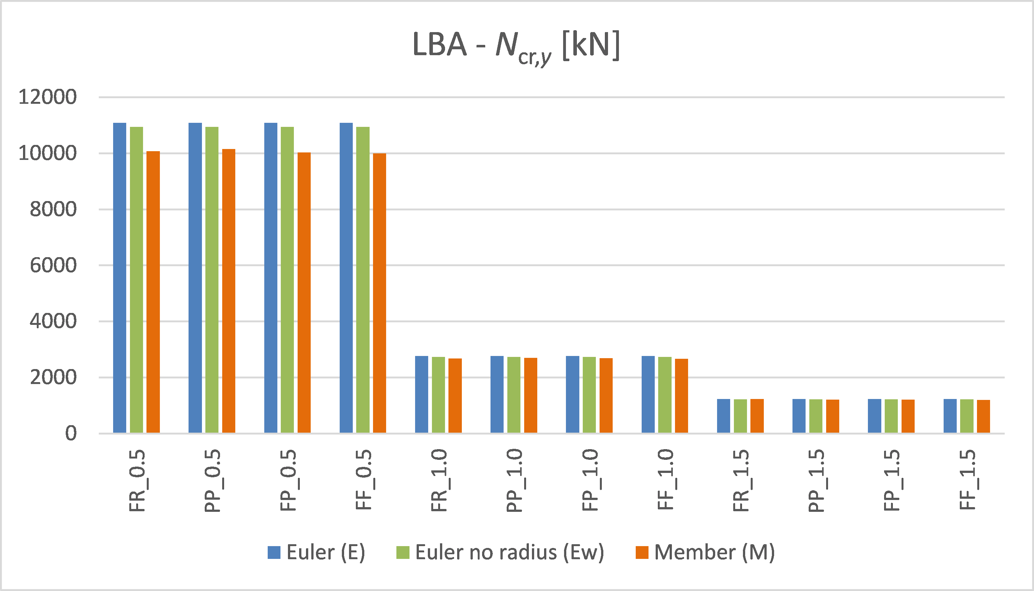
Chart 1: Critical load values – axis y-y
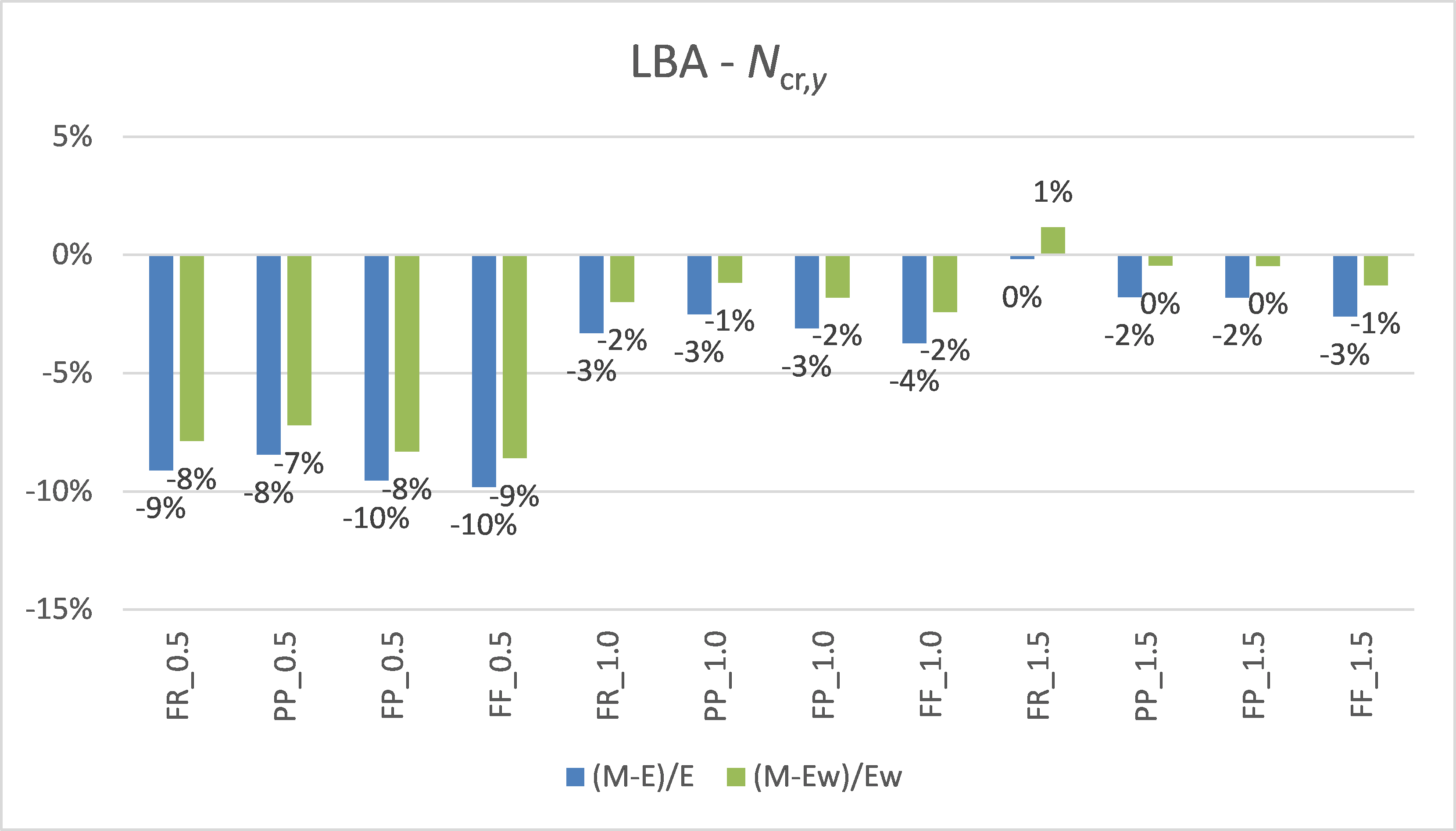
Chart 2: Critical load comparison – axis y-y
Note the difference between the blue and green columns in the chart above. This is the influence of the missing radii and it is shown to be a difference of under 2 % for strong axis buckling.
Weak axis buckling
The results for weak axis buckling are summarized in the table below.
Tab. 2: Resulting critical loads – axis z-z
The results of LBA are slightly conservative (< 3 %) for columns with low relative slenderness. For higher relative slenderness, the critical loads are very close to the expected analytical value.
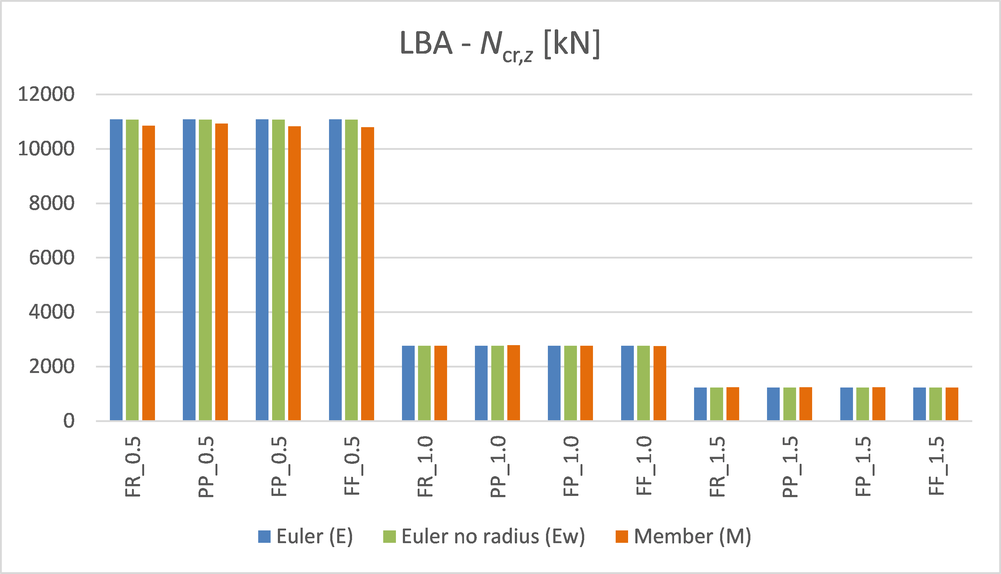
Chart 3: Critical load values – axis z-z
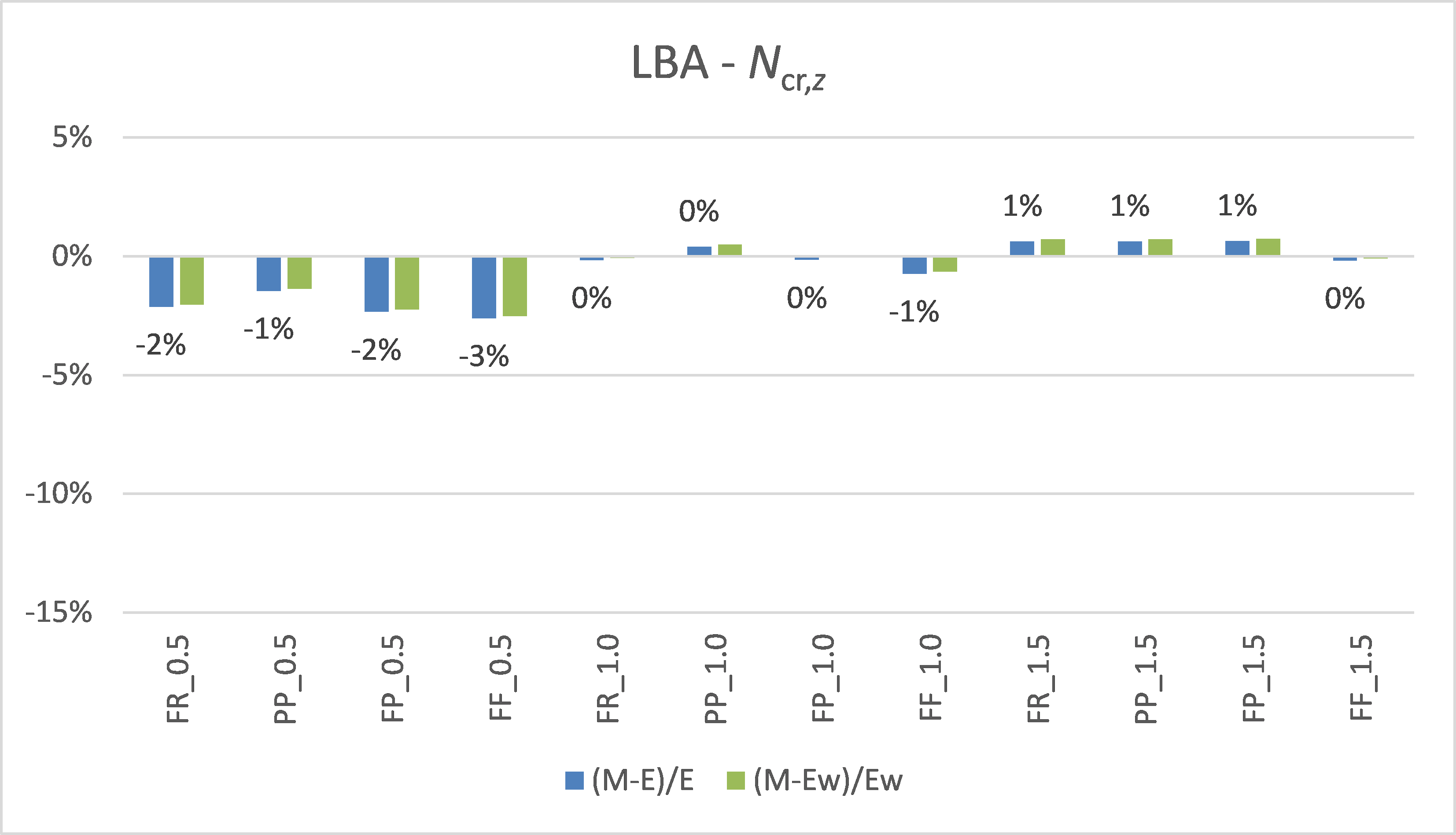
Chart 4: Critical load comparison – axis z-z
Note that there is almost no difference between the blue and green columns in the chart above. The influence of the missing radii is shown to be negligible for weak axis buckling.